Benchtop Spectrophotometry of Solutions

Benchtop Spectrophotometry of Solutions in Transmission Mode (T-mode)

The benchtop spectrophotometer was invented by Arnold Beckman and his colleagues at the National Technologies Laboratories in 1940. Beckman, a professor at California Institute of Technology, started NTL in the 1930s, dedicated to designing, producing and selling sophisticated scientific instruments. NTL would later become Beckman Instruments. The development of the earliest model spectrophotometer, the DU, was led by project leader Howard Cary. The invention of the spectrophotometer has been described as one of the most significant in the biosciences. Howard Cary, with two colleagues, later started the Applied Physics Corporation, renamed Cary Instruments (subsequently purchased by Varian Associates). They are also a major supplier of benchtop spectrophotometers.

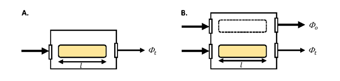
Designs of spectrophotometers vary between manufacturers and the differences can impact the accuracy of the derived absorption due to variability in the measurements of ${\Phi }_o$ and ${\Phi }_t$. Because these instruments were developed for non-scattering solutions, users make modifications to optimize scattering collection and to correct for scattering not detected. Spectrophotometers come in single beam- and dual-beam models (Figure 1). The incident radiant power, generated by a lamp, passes through a monochrometer (not shown) so that light within a narrow spectral band enters the sampling chamber. In the single-beam mode, the incident and transmitted radiant power are determined from two separate scans, the first with a reference material in the sample chamber (e.g., pure water) and the second with the sample in the sample chamber (e.g., filtered seawater). In the dual-beam mode, the incident and transmitted radiant power are measured nearly simultaneously using a beam splitter between the diffraction monochrometer and the sample chamber. Similarly in the dual beam model, there is a mirror system to direct the incident and transmitted beams to the detector in an alternating fashion as the instrument scans.

Spectrophotometers output their signal in absorbance ($Abs$, sometimes called the optical density, although the International Union of Pure and Applied Chemistry (IUPAC) recommended against this term in the Compendium of Chemical Terminology). Absorbance $Abs$ is the log base ten of the absorptance $A$:

and therefore $A=10^{Abs}$. So

So absorption is computed from the spectrophotometric absorbance as

where the constant 2.303 is the natural logarithm of 10, and $\ell$ is the geometric pathlength of the cuvette in units of meters. In order to maintain the adherence to Beer’s Law so that the absorptance is linearly related to both the concentration of the absorbing material and to the geometric pathlength (i.e., there is no self shading), it is recommended that the absorptance (optical density) from the spectrophotometer be maintained within the range 0.1 to 0.4. This is equivalent to tranmittances of approximately 80% and 40%, respectively.

The best practice for spectrophotometry of solutions is the employ a dual beam model to minimize uncertainty in the lamp intensity (${\Phi }_o$, Fig. 1B). When running multiple samples, the material in the reference cuvette can undergo changes such as increases in temperature due to the lamp relative to the sample. Rather than changing the reference material with every sample, which comes with its own set of handling uncertainties, it is recommended to run the dual beam mode without a cuvette in the reference path (i.e., remove the dashed line cuvette in Fig. 1B) and follow either:

1.

Automatic baseline correction, which consists of the following scan order:

(a)

baseline scan with nothing in the reference beam and reference material in the sample cuvette (most spectrophotometers will subtract this automatically from the sample scans)

(b)

without opening the sample compartment, immediately scan again as a sample, this is essentially running the baseline against itself (a zero scan). The expectation is that the result is close to zero ( the uncertainty of the instrument, 0.0001) and spectrally flat

(c)

3-5 blank scans (again with nothing in the reference beam and with new reference material in the sample cuvette)

(d)

Alternating between sets of 5-6 sample scans and a blank scan

2.

Post processing baseline correction, which consists of the following scan order:

(a)

3-5 blank scans, each with new reference material in the sample cuvette

(b)

Alternating between sets of 5-6 sample scans and a blank scan

The upside of method (1) is the ability to easily view the variability in the sample scans without having to visually remove the baseline in real time. Additionally, it allows for quantification of the instrument resolution with the zero scan. The downside is that a single scan is used as a baseline, and the average of the 3-5 initial blank scans provides the uncertainty in that baseline. The upside of method (2) is that the mean blank is used as the baseline correction but the downside is that it can be difficult to visually analyze the sample scans as they contain the blank signal in them. Regardless of method, the time series of blank scans is used to quantify the drift of the instrument. If significant the time course of the blank signal must be removed from the samples as part of the complete baseline correction.