Geometry

This page develops the mathematical tools needed to specify directions and angles in three-dimensional space. These mathematical concepts are fundamental to the specification of how much light there is and what direction it is traveling.

Coordinate Systems and Directions

Locations and directions will be specified with reference to particular coordinate systems chosen to be convenient for the problem at hand. These coordinate systems can be “global” or “ocean” systems that are fixed once and for all in their spatial orientation, or they can be “local” systems determined by the instantaneous direction of light propagation.

Global coordinate systems

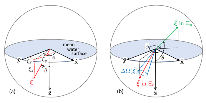
The most common ocean system is defined as follows. Let let $\widehat{x},ŷ$ and $ẑ$ be three mutually perpendicular unit vectors that define a right-handed Cartesian coordinate system. Let the depth $z$ be measured positive downward from 0 at the mean sea surface, as is customary in oceanography. The unit direction vector $ẑ$ thus points downward. For problems involving sea surface waves it is convenient to resolve the waves into “along-wind” and “cross-wind” components (see the pages on Cox-Munk sea-surface slope statistics and modeling sea surfaces). This is most easily done if $\widehat{x}$ is chosen to be in the direction that the wind is blowing over the ocean surface, i.e. $\widehat{x}$ points downwind. The cross-wind direction is then given by the cross (or vector) product $ŷ=ẑ\times \widehat{x}$. This defines the “wind-based” coordinate system used in the HydroLight radiative transfer code. If the problem at hand required the analysis of Sun glint on the sea surface as seen from an airplane, then it would be convenient to use a “Sun-based” system with $\widehat{x}$ pointing towards or away from the Sun and $ẑ$ pointing upward, away from the mean sea surface (see Fig. 2 of the Cox-Munk page). No matter how chosen, the $\left(\widehat{x},ŷ,ẑ\right)$ directions remain fixed in space for the given problem.

Given a global coordinate system, a direction in space is specified as follows. Let $\widehat{\xi }$ denote a unit vector pointing in the desired direction. The vector $\widehat{\xi }$ has components ${\xi }_x,{\xi }_y$ and ${\xi }_z$ in the $\widehat{x},ŷ$ and $ẑ$ directions, respectively. We can therefore write

$$\widehat{\xi }={\xi }_x\widehat{x}+{\xi }_yŷ+{\xi }_zẑ,$$

or just $\widehat{\xi }=\left({\xi }_x,{\xi }_y,{\xi }_z\right)$ for notational convenience. Note that because $\widehat{\xi }$ is of unit length, its components satisfy ${\xi }_x^2+{\xi }_y^2+{\xi }_z^2=1.$

An alternative description of $\widehat{\xi }$ is given by the angles $𝜃$ and $\varphi$, defined as shown in Fig. 1. The polar angle $𝜃$ is measured from the direction of $ẑ$, and the azimuthal angle $\varphi$ is measured positive counterclockwise from $\widehat{x}$, when looking toward the origin along $ẑ$ (i.e. when looking in the $-ẑ$ direction). For downward directions (the red arrow in the figure), $𝜃<\pi ∕2$; for upward directions (the green arrow in Panel (b)), $𝜃>\pi ∕2$. The connection between $\widehat{\xi }=\left({\xi }_x,{\xi }_y,{\xi }_z\right)$ and $\widehat{\xi }=\left(𝜃,\varphi \right)$ is obtained by inspection of Panel (a) of Fig. 1:

$$\begin{array}{llll}\hfill {\xi }_x=& sin𝜃cos\varphi & \hfill & \\ \hfill {\xi }_y=& sin𝜃sin\varphi & \hfill \text{(1)}\\ \hfill {\xi }_z=& cos𝜃& \hfill & \end{array}$$

where $𝜃$ and $\varphi$ lie in the ranges $0\le 𝜃\le \pi$ and $0\le \varphi <2\pi$. The inverse transformation is

$$\begin{array}{llll}\hfill 𝜃=& {cos}^{-1}\left({\xi }_z\right)& \hfill & \\ \hfill \varphi =& {tan}^{-1}\left(\frac{{\xi }_y}{{\xi }_x}\right)& \hfill \text{(2)}\end{array}$$

The polar coordinate form of $\widehat{\xi }$ could be written as $\widehat{\xi }=\left(r,𝜃,\varphi \right),$ but since the length of $r$ is 1, we can drop the radial coordinate for brevity.

---

---

Another useful description of $\widehat{\xi }$ is obtained using the cosine parameter

$$\mu \equiv cos𝜃={\xi }_z.$$

(3)

The components of $\widehat{\xi }=\left({\xi }_x,{\xi }_y,{\xi }_z\right)$ and $\widehat{\xi }=\left(\mu ,\varphi \right)$ are related by

$$\begin{array}{llll}\hfill {\xi }_x=& {\left(1-{\mu }^2\right)}^{1∕2}cos\varphi & \hfill & \\ \hfill {\xi }_y=& {\left(1-{\mu }^2\right)}^{1∕2}sin\varphi & \hfill \text{(4)}\\ \hfill {\xi }_z=& \mu ,& \hfill & \end{array}$$

with $\mu$ and $\varphi$ in the ranges $-1\le \mu \le 1$ and $0\le \varphi <2\pi$. Hence a direction $\widehat{\xi }$ can be represented in three equivalent ways: as $\left({\xi }_x,{\xi }_y,{\xi }_z\right)$ in Cartesian coordinates, and as $\left(𝜃,\varphi \right)$ or $\left(\mu ,\varphi \right)$ in polar coordinates.

The scalar (or dot) product between two direction vectors ${\widehat{\xi }}^{\prime }$ and $\widehat{\xi }$ can be written as

$${\widehat{\xi }}^{\prime }\cdot \widehat{\xi }=\left|{\widehat{\xi }}^{\prime }\right|\left|\widehat{\xi }\right|cos\psi =cos\psi ,$$

where $\psi$ is the angle between directions ${\widehat{\xi }}^{\prime }$ and $\widehat{\xi }$, and $\left|\widehat{\xi }\right|$ denotes the (unit) length of vector $\widehat{\xi }$. The scalar product expressed in Cartesian-component form is

$${\widehat{\xi }}^{\prime }\cdot \widehat{\xi }={{\xi }^{\prime }}_x{\xi }_x+{{\xi }^{\prime }}_y{\xi }_y+{{\xi }^{\prime }}_z{\xi }_z.$$

Equating these representations of ${\widehat{\xi }}^{\prime }\cdot \widehat{\xi }$ and recalling Eqs. (1) and (4) leads to

$$\begin{array}{llll}\hfill cos\psi =& {\xi }_x^{\prime }{\xi }_x+{\xi }_y^{\prime }{\xi }_y+{\xi }_z^{\prime }{\xi }_z& \hfill & \\ \hfill =& cos{𝜃}^{\prime }cos𝜃+sin{𝜃}^{\prime }sin𝜃cos\left({\varphi }^{\prime }-\varphi \right)& \hfill \text{(5)}\\ \hfill =& {\mu }^{\prime }\mu +\sqrt{1-{{\mu }^{\prime }}^2}\sqrt{1-{\mu }^2}cos\left({\varphi }^{\prime }-\varphi \right)& \hfill & \end{array}$$

Equation (5) gives very useful connections between the various coordinate representations of ${\widehat{\xi }}^{\prime }$ and $\widehat{\xi }$, and the included angle $\psi$. In particular, this equation allows us to compute the scattering angle $\psi$ when light is scattered from an incident direction ${\widehat{\xi }}^{\prime }$ to a final direction $\widehat{\xi }$.

The set of all directions $\widehat{\xi }$ is called the unit sphere of directions, which is denoted by $\Xi$. Referring to polar coordinates, $\Xi$ therefore represents all $\left(𝜃,\varphi \right)$ values such that $0\le 𝜃\le \pi$ and $0\le \varphi <2\pi$. Two subsets of $\Xi$ frequently employed in optical oceanography are the downward (subscript d) and upward (subscript u) hemispheres of directions, ${\Xi }_d$ and ${\Xi }_u$, defined by

$$\begin{array}{llll}\hfill {\Xi }_d& \equiv all\left(𝜃,\varphi \right)suchthat0\le 𝜃\le \pi ∕2and0\le \varphi <2\pi ,& \hfill & \\ \hfill {\Xi }_u& \equiv all\left(𝜃,\varphi \right)suchthat\pi ∕2<𝜃\le \pi and0\le \varphi <2\pi .& \hfill & \end{array}$$

Some authors use the notation $2{\pi }_d$ for ${\Xi }_d$ and $2{\pi }_u$ for ${\Xi }_u$ because these hemispheres of directions contain $2\pi$ steradians of solid angle.

Local coordinate systems

In Monte Carlo ray tracing calculations, for example, it is necessary to specify the polar and azimuthal scattering angles of a scattered ray relative to the direction of the unscattered ray. This requires defining a local (at the end point of the unscattered ray) Cartesian system “centered” on the direction of the unscattered ray, rather than on a fixed $ẑ$ direction. A local system that meets the needs of Monte Carlo ray tracing can be defined as follows.

Referring to Fig. 2, let $R^{\prime }=\left|R^{\prime }\right|{\widehat{\xi }}^{\prime }$ denote a light ray with starting point $r_1=\left(x_1,y_1,z_1\right)$ and ending point $r_2=\left(x_2,y_2,z_2\right)$ in a global coordinate system. $\left|R^{\prime }\right|$ is the length of the vector $R^{\prime }$, which is traveling in direction ${\widehat{\xi }}^{\prime }=\left({𝜃}^{\prime },{\varphi }^{\prime }\right)$ in the global system. Now suppose that this ray scatters at point $r_2$ to create a new ray $R$, which ends at poinr $r_3$. To describe that scattering, it is necessary to define a local (at the point of scattering $r_2$) coordinate system for the scattering calculations. The scattering angles $\psi$ and $\alpha$ (computed as described on page Probability Functions will then be applied in this system to determine the direction of the scattered ray $R$ relative to the unscattered ray $R^{\prime }$.

---

---

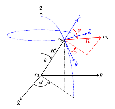
In the ocean system, ray $R^{\prime }$ has components $\left(R_x^{\prime },R_y^{\prime },R_z^{\prime }\right)$:

$$\begin{array}{llll}\hfill R^{\prime }=& R_x^{\prime }\widehat{x}+R_y^{\prime }ŷ+R_z^{\prime }ẑ& \hfill & \\ \hfill =& R^{\prime }sin𝜃cos\varphi \widehat{x}+R^{\prime }sin𝜃sin\varphi ŷ+R^{\prime }cos𝜃ẑ,& \hfill \text{(6)}\end{array}$$

where the Cartesian components $R_x^{\prime }$ etc., in terms of spherical coordinates come from Eq (1).

A convenient local coordinate system $\left(\widehat{𝜃},\widehat{\varphi },\widehat{r}\right)$ for scattered rays is constructed as follows. The radial unit vector

$$\widehat{r}=\frac{R^{\prime }}{\left|R^{\prime }\right|}=\frac{r_2-r_1}{|r_2-r_1|}$$

is in the same direction as the initial ray $R^{\prime }$. The azimuthal unit vector $\widehat{\varphi }$ is defined by the cross product of the ocean coordinate system $ẑ$ and the incident vector’s direction:

$$\widehat{\varphi }=\frac{ẑ\times \widehat{r}}{|ẑ\times \widehat{r}|}.$$

This vector points in the direction of increasing $\varphi$ values. (If the unscattered vector is in the same direction as $ẑ$, the direction of $\widehat{\varphi }$ can be chosen at random.) The polar unit vector is then given by

$$\widehat{𝜃}=\widehat{\varphi }\times \widehat{r}.$$

This vector points in the direction of increasing $𝜃$ values. (If you think of point $r_2$ as being on the surface of the Earth, then $\widehat{𝜃}$ points south, $\widehat{\varphi }$ points east, and $\widehat{r}$ is straight up.) The $\left(\widehat{𝜃},\widehat{\varphi },\widehat{r}\right)$ system is then an orthogonal system of coordinates in which the scattering angles $\psi$ and $\alpha$ can be applied to define the direction of the scattered ray. However, these directions are not fixed in the ocean system; they depend on the direction of the unscattered ray $R^{\prime }$.

After the direction of the scattered ray has been determined in the local $\left(\widehat{𝜃},\widehat{\varphi },\widehat{r}\right)$ system, the scattered ray direction must be specified in terms of $\left(𝜃,\varphi \right)$ in the global system, so that the scattering process can be repeated.

Similarly, in calculations involving polarization, a local Cartesian system is needed to resolve the components of the polarization relative to some reference plane. This reference plane can be either the meridian plane, which is the plane containing $ẑ$ and the direction of propagation; or the scattering plane, which is the plane containing the incident and final directions of the scattered light (see Figs. 1 and 2 on the Polarization: Scattering Geometry page). Again, the appropriate local coordinate system depends on the direction of propagation of the light.

Solid Angle

Closely related to the specification of directions in three-dimensional space is the concept of solid angle, which is an extension of two-dimensional angle measurement. As illustrated in panel (a) of Fig. 3, the plane angle $𝜃$ between two radii of a circle of radius $r$ is

The angular measure of a full circle is therefore $2\pi$ rad. In panel (b) of Fig. 3, a patch of area $A$ is shown on the surface of a sphere of radius $r$. The boundary of $A$ is traced out by a set of directions $\widehat{\xi }$. The solid angle $\Omega$ of the set of directions defining the patch $A$ is by definition

---

---

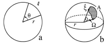
Since the area of a sphere is $4\pi r^2$, the solid angle measure of the set of all directions is $\Omega \left(\Xi \right)=4\pi sr$. Note that both plane angle and solid angle are independent of the radii of the respective circle and sphere. Both plane and solid angle are dimensionless numbers. However, they are given “units” of radians and steradians, respectively, to remind us that they are measures of angle.

Consider a simple application of the definition of solid angle and the observation that a full sphere has $4\pi sr$. The area of Brazil is $8.5\cdot 10^{6}k{m}^2$ and the area of the earth’s surface is $5.1\cdot 10^{8}k{m}^2$. The solid angle subtended by Brazil as seen from the center of the earth is then $4\pi 8.5\cdot 10^6∕5.1\cdot 10^8=0.21sr$.

---

---

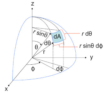
The definition of solid angle as area on the surface of a sphere divided by radius of the sphere squared gives us a convenient form for a differential element of solid angle, as needed for computations. The blue patch shown in Fig. 4 represents a differential element of area $dA$ on the surface of a sphere of radius $r$. Simple trigonometry shows that this area is $dA=\left(rsin𝜃d\varphi \right)\left(rd𝜃\right).$ Thus the element of solid angle $d\Omega \left(\widehat{\xi }\right)$ about the direction $\widehat{\xi }=\left(𝜃,\varphi \right)$ is given in polar coordinate form by

$$\begin{array}{llll}\hfill d\Omega \left(\widehat{\xi }\right)=& \frac{dA}{r^2}=\frac{\left(rsin𝜃d\varphi \right)\left(rd𝜃\right)}{r^2}=sin𝜃d𝜃d\varphi & \hfill & \\ \hfill =& d\mu d\varphi \left(sr\right).& \hfill \text{(7)}\end{array}$$

(The last equation is correct even though $d\mu =dcos𝜃=-sin𝜃d𝜃$. When the differential element is used in an integral and variables are changed from $\left(𝜃,\varphi \right)$ to $\left(\mu ,\varphi \right)$, the Jacobian of the transformation involves an absolute value.)

Example: Solid angle of a spherical cap

To illustrate the use of Eq. (7), let us compute the solid angle of a “polar cap” of half angle $𝜃$, i.e. all $\left({𝜃}^{\prime },{\varphi }^{\prime }\right)$ such that $0\le {𝜃}^{\prime }\le 𝜃$ and $0\le {\varphi }^{\prime }<2\pi$. Integrating the element of solid angle over this range of $\left({𝜃}^{\prime },{\varphi }^{\prime }\right)$ gives

$${\Omega }_{\text{cap}}={\int \; <!--nolimits-->}_{{\varphi }^{\prime }=0}^{2\pi }{\int \; <!--nolimits-->}_{{𝜃}^{\prime }=0}^{𝜃}sin{𝜃}^{\prime }d{𝜃}^{\prime }d{\varphi }^{\prime }=2\pi \left(1-cos𝜃\right),$$

(8)

or

$${\Omega }_{\text{cap}}={\int \; <!--nolimits-->}_{{\varphi }^{\prime }=0}^{2\pi }{\int \; <!--nolimits-->}_{{\mu }^{\prime }=\mu }^{1}d{\mu }^{\prime }d{\varphi }^{\prime }=2\pi \left(1-\mu \right).$$

(9)

Note that ${\Xi }_d$ and ${\Xi }_u$ are special cases of a spherical cap (having $𝜃=\pi ∕2$), and that $\Omega \left({\Xi }_d\right)=\Omega ({\Xi }_u$) = $2\pi sr$.

Dirac Delta functions

It is sometimes convenient to specify directions using the Dirac delta function, $\delta \left(\widehat{\xi }-{\widehat{\xi }}_o\right)$. This peculiar mathematical construction is defined (for our purposes) by

$$\delta \left(\widehat{\xi }-{\widehat{\xi }}_o\right)\equiv 0if\widehat{\xi }\ne {\widehat{\xi }}_o,$$

(10)

and

$${\int \; <!--nolimits-->}_{\Xi }f\left(\widehat{\xi }\right)\delta \left(\widehat{\xi }-{\widehat{\xi }}_o\right)d\Omega \left(\widehat{\xi }\right)\equiv f\left({\widehat{\xi }}_o\right).$$

(11)

Here $f\left(\widehat{\xi }\right)$ is any function of direction. Note that $\delta \left(\widehat{\xi }-{\widehat{\xi }}_o\right)$ simply “picks out” the particular direction ${\widehat{\xi }}_o$ from all directions in $\Xi$. Note also in Eq. (11) that because the element of solid $d\Omega \left(\widehat{\xi }\right)$ has units of steradians, it follows that $\delta \left(\widehat{\xi }-{\widehat{\xi }}_o\right)$ has units of inverse steradians.

Equations (10) and (11) are a symbolic definition of $\delta$. The mathematical representation of $\delta \left(\widehat{\xi }-{\widehat{\xi }}_o\right)$ in spherical coordinates $(𝜃$,$\varphi )$ is

$$\delta \left(\widehat{\xi }-{\widehat{\xi }}_o\right)=\frac{\delta \left(𝜃-{𝜃}_o\right)\delta \left(\varphi -{\varphi }_o\right)}{sin𝜃}\left(s{r}^{-1}\right),$$

(12)

where $\widehat{\xi }=\left(𝜃,\varphi \right),{\widehat{\xi }}_o=\left({𝜃}_o,{\varphi }_o\right)$, and

$$\begin{array}{llll}\hfill {\int \; <!--nolimits-->}_0^{\pi }f\left(𝜃\right)\delta \left(𝜃-{𝜃}_o\right)d𝜃\equiv & f\left({𝜃}_o\right)& \hfill & \\ \hfill {\int \; <!--nolimits-->}_0^{2\pi }f\left(\varphi \right)\delta \left(\varphi -{\varphi }_o\right)d\varphi \equiv & f\left({\varphi }_o\right).& \hfill & \end{array}$$ Note that the $sin𝜃$ in the denominator of Eq. (12) is necessary to cancel the $sin𝜃$ factor in the element of solid angle when integrating in polar coordinates. Thus

$$\begin{array}{llll}\hfill & {\int \; <!--nolimits-->}_{\Xi }f\left(\widehat{\xi }\right)\delta \left(\widehat{\xi }-{\widehat{\xi }}_o\right)d\Omega \left(\xi \right)=& \hfill & \\ \hfill & {\int \; <!--nolimits-->}_0^{2\pi }{\int \; <!--nolimits-->}_0^{\pi }f\left(𝜃,\varphi \right)\frac{\delta \left(𝜃-{𝜃}_o\right)\delta \left(\varphi -{\varphi }_o\right)}{sin𝜃}sin𝜃d𝜃d\varphi =& \hfill & \\ \hfill & f\left({𝜃}_o,{\varphi }_o\right)=f\left({\widehat{\xi }}_o\right).& \hfill & \end{array}$$

Likewise, we can write

$$\delta \left(\widehat{\xi }-{\widehat{\xi }}_o\right)=\delta \left(\mu -{\mu }_o\right)\delta \left(\varphi -{\varphi }_o\right)\left(s{r}^{-1}\right),$$

(13)

where

$${\int \; <!--nolimits-->}_{-1}^{1}f\left(\mu \right)\delta \left(\mu -{\mu }_o\right)d\mu \equiv f\left({\mu }_o\right).$$