Page updated:
March 22, 2021
Author: Curtis Mobley
View PDF
A Turbulence-Generated Surface
This page illustrates the generation of random water surfaces beginning with the analytical autocovariance function of Horoshenkov et al. (2013),
| (1) |
This particular autocovariance has an analytical spectrum,
| (2) |
which was computed on the Autocovariance Functions: Theory page. Thus, for surface generation, the two-sided spectrum of Eq. (2) simply replaces the two-sided Pierson-Moskowitz spectrum used on the previous page, and the surface-generation calculations proceed as described in the previous pages. The autocovariance function is then not needed. However, if only the autocovariance is known or measured, then the needed variance spectrum must be obtained via the Wiener-Khinchin theorem. In the present study, knowing both the autocovariance and the spectral density as analytical functions provides a powerful check on the discrete numerical calculations of the same quantities.
The application of the above results is straightforward. If only the autocorrelation, rather than the autocovariance, is given, then a separate value of the surface elevation variance must be known. For the Horoshenkov study, a typical value of the surface variance is . (This is extremely small by oceanographic standards, but the surface waves in the Horoshenkov laboratory experiment had amplitudes of order 1 mm.) The previously cited parameter values of and are used here. Since the characteristic spatial scales of and are of order 0.2 m, a spatial region of length should be adequate to capture the spatial features of these surfaces. An value of 1024 then gives the smallest resolvable wavelength as , which is the scale of capillary waves. (Capillary waves have wavelengths in the range of a few millimeters to 2 cm.)
Figure 1 shows an example simulation based on the Horoshenkov variance spectrum (2). The layout is the same as for the Pierson-Moskowitz figures on the previous pages. Panel (d) of the figure contains three autocovariance plots: The green curve is the inverse DFT of the sampled variance spectrum, which is shown in green in Panel (b). The red curve is the ensemble average autocovariance of 1000 water surface simulations. The purple curve is the theoretical autocovariance of Eq. (1). These three curves are indistinguishable at the scale of this plot. This nearly perfect agreement between autocovariance derived in three different ways indicates that the various numerical calculations are almost without doubt being done correctly.
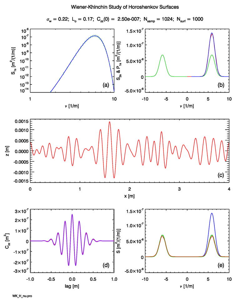
The red curve in Panel (e) of the plot shows the variance spectrum derived via the Wiener-Khinchin theorem as the DFT of the ensemble-average autocovariance (the red curve in Panel (d)). Again, this curve is almost indistinguishable from the theoretical autocovarinace, which is shown in green. Again, this agreement indicates that the DFTs are being computed correctly.
Two-dimensional Water Surfaces
The IDL codes used on previous pages for generation of two-dimensional, time-independent water surfaces are formulated using a one-sided, two-dimensional elevation variance spectrum of the form (recall Eq. 4 of the Wave Variance Spectra: Examples)
| (3) |
Here is a one-sided omnidirectional spectrum and is a nondimensional spreading function. To generate a 2-D, time-independent surface using the Horoshenkov model, the two-sided omnidirectional spectrum of Eq. (??) is multiplied by 2 to obtain a one-sided spectrum, which the IDL code evaluates only for the non-negative values, i.e. for . The code then divides the result by 2 to get a two-sided spectrum and evaluates the half plane of values by symmetry. Thus it is easy to replace an omnidirectional oceanographic spectrum with that of Horoshenkov. There remains only the issue of what to use for a spreading function. There is no information about the spreading functions of turbulence-generated waves in the Horoshenkov et al. paper. There is no doubt some flow-induced difference in the waves in the “down-river” vs “cross-river” directions, just as there is in the “down-wind” vs “cross-wind” directions for wind-generated waves. However, pending further information on that difference, it is probably reasonable to use a frequency-independent, isotropic spreading function, . With that assumption, two-dimensional surfaces can be generated.
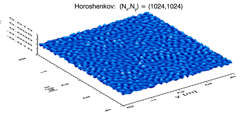
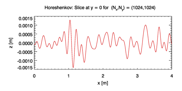
Figure 2 shows an example two-dimensional, turbulence-generated surface created with the , and values used for Fig. 1. This particular 2-D surface realization has an elevation variance of , which is close to the value of value used as input to the Horoshenkov spectrum. It is also noted that along any slice through the surface, there are about two dozen “bumps” in 4 m, just as seen in the 1-D surface realization of Fig. 1. Figure 3 shows the slice through the 2-D surface at . This surface is qualitatively like that of the middle panel of Fig. 1. These results indicate that the 2-D calculations are correct.
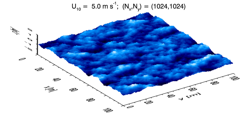
The visual appearance of the Horoshenkov surface is strikingly different from the wind-generated sea surface seen in Fig. 4, which is for a wind speed. In these plots, the surfaces have a factor-of-8 difference in the scaling of the surface elevation relative to the horizontal: 0.02 m vertical to 4 m horizontal = 0.005 for the Horoshenkov surface compared 4 m to 100 m = 0.04 for the wind-blown surface. This is purely for the visual appearance of the 3D perspective plots. The Horoshenkov surface is actually quite smooth, with an average wave facet slope of only about 0.6 deg. The wind-blown surface has an average slope angle of about 3.7 deg in the along-wind direction and 2.9 deg in the cross-wind direction. (Keep in mind that for this simulation , so the smallest resolvable wave has a wavelength of about 20 cm. Thus the smallest waves, which can have large slopes, are not resolved. An actual sea surface will therefore have larger average slopes.) Thus the Horoshenkov surface is smoother than the wind-blown surface, which suggests that turbulence-generated water surfaces may have significantly different optical reflectances than wind-generated surfaces. That hypothesis could be tested by ray tracing calculations based on surfaces like those of Figs. 2 and 4.
 See comments posted for this page and leave your own.