Page updated:
May 11, 2021
Author: Curtis Mobley
View PDF
Polarization
Radiance leaving the top of the atmosphere can be strongly polarized even though the sunlight incident onto the TOA is unpolarized. This is because scattering by atmospheric constituents, reflection by the sea surface, and scattering within the water all can generate various states of polarization from unpolarized radiance. Although remote sensing as considered here is based on the total TOA radiance without regard to its state of polarization, many instruments are sensitive to polarization. Therefore, the total TOA radiance they measure may depend on the state of polarization of the TOA radiance and the orientation of the instrument relative to the plane of linear polarization. Correction for these effects is required so that instruments give consistent measurements of the total TOA radiance.
The MODIS sensors are polarization sensitive. MODIS radiance measurements vary by up to for totally linearly polarized radiance, depending of the orientation of the sensor relative to the plane of polarization. This amounts to about differences in measured TOA radiances for typical values of atmospheric polarization Meister et al. (2005). These effects must be accounted for in order to achieve the desired 0.5% accuracy in measured TOA radiance. Similarly, the VIIRS instrument polarization sensitivity is 1-2% and requires a polarization correction. SeaWiFS was by design not very sensitive to polarization (), and no polarization correction was applied.
The state of polarization is described by the four-component Stokes vector , where superscript denotes transpose, is the total radiance without regard for its state of polarization, specifies the linear polarization resolved in planes parallel and perpendicular to a conveniently chosen reference plane, specifies the polarization resolved in planes oriented to the reference plane, and specifies the right or left circular polarization. The choice of the reference plane for specification of the and components is arbitrary and can be made for convenience. The direction of propagation of the radiance is given by a unit vector , so that the Stokes vector can be written as when it is desired to indicate both its components and direction. Direction can be specified by the polar () and azimuthal () directions in a spherical coordinate system as shown in Fig. 1. In that figure, and are unit vectors specified by the directions of increasing ( at the pole or direction in a cartesian coordinate system) and increasing ( in a conveniently chosen azimuthal direction such as pointing east or toward the Sun).
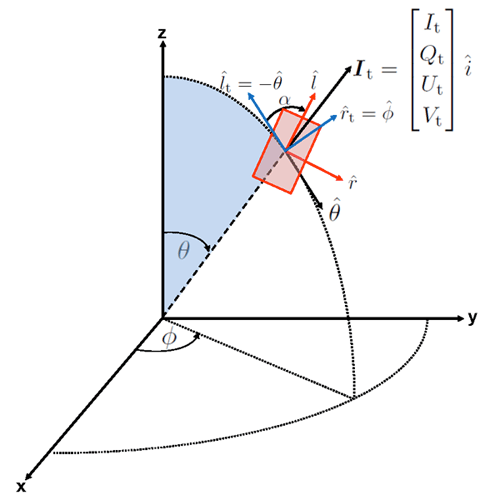
In the geophysical setting, it is customary to define the Stoke vector components and with reference to a plane defined by the normal to the sea surface and the direction of propagation of the radiance. This plane is known as the meridional plane and is partly shaded in light blue in Fig. 1. Following the notation and choices of Gordon et al. (1997a), let be the reference direction perpendicular to the meridional plane, and let be the reference direction parallel to the meridional plane. The direction of propagation of the radiance to be measured is then . The total TOA radiance resolved in these directions is denoted .
This radiance is being measured by a sensor illustrated by the red rectangle in Fig. 1. The Stokes vector measured by that sensor has its and components resolved along perpendicular () and parallel () directions chosen for convenience relative to the orientation of the sensor. The sensor will measure the TOA radiance as a Stokes vector . For an incident radiance , the optical system comprising the sensor itself and any associated optical components (mirrors, lenses, etc.) will convert the incient radiance into a measured value given by , where is the Mueller matrix that describes the optical properties of the sensor optical system. is defined relative to the sensor reference directions and . In order for to operate on the TOA radiance , which is defined with reference directions and , must first be transformed (rotated) from the meridional-based , system to the sensor-based , system.
Let be the angle between the parallel reference directions for and for the sensor. With the choice of being positive for clockwise rotations from to as seen looking “into the beam” (looking in the direction), the transformation is given by the rotation matrix
| (1) |
Thus, the radiance as measured by the sensor is
| (2) |
It is important to note that the radiance measured by the sensor, depends both on the ”true” TOA radiance , the sensor optical properties via , and the orientation of the sensor relative to the local meridional plane. is fixed for a given sensor, but and change from moment to moment as the sensor orbits and views the TOA radiance in different locations and directions. (To be exact, there are long-term changes to caused by degradation of the sensor optical surfaces. These changes are monitored on-orbit and corrected by a cross-calibration technique.)
The quantity of interest here is the measured TOA radiance magnitude, which is given by the first element of the Stokes vector. Using (1) in Eq. (2) gives this to be
Clearly, if and all elements of other than the element are zero, then the sensor is not sensitive to the state of polarization and . Physical arguments and numerical simulation show the circular polarization of the TOA radiance is very small: . This term is therefore neglected in the present correction algorithm. It is customary to define the elements of the reduced Mueller matrix by . Similarly defining reduced Stokes vector element by and , Eq. (3) becomes
Gordon et al. (1997a) give the general procedure for measuring and in the laboratory. Meister et al. (2005) give the details of these measurements for the MODIS sensors. These quantities, which specify the polarization sensitivity of the instrument, are determined before the instrument is launched; they are thus known. Angle is determined by the orbit and pointing geometry of the sensor. It remains to determine the elements of .
Following Eq. (3) of the Problem Formulation page, the total TOA polarized radiance can be decomposed as
| (5) |
Here, as before, the Rayleigh (R), aerosol (a), and Rayleigh-aerosol (Ra) radiances are at the TOA; the glint (g), whitecap (wc), and water-leaving (w) radiances are at the sea surface. The surface values are transmitted to the TOA via the appropriate direct () and diffuse () transmittances. According to Eq. (2), each of these radiances must be known in order to predict what the sensor will measure for a given TOA radiance and, thereby, to determine the correction needed to account for sensor polarization effects.
The surface-glint and atmospheric polarization contributions to the TOA signal are computed separately. Sea-surface glint can be highly polarized. This glint contribution to the TOA signal is computed using a vector radiative transfer code assuming a Rayleigh-scattering atmosphere above a rough Fresnel-reflecting ocean surface (Gordon and Wang (1992), Wang (2002), Meister et al. (2005)). The water-leaving radiance is at most 10% of the TOA total, and the whitecap contribution is generally even less. These two terms are therefore ignored in the present development. The effect of aerosols and Rayleigh-aerosol interactions depends on the particle size distribution and concentration of the aerosols, which are unknown during atmospheric correction. Fortunately, numerical simulations show that the Rayleigh contribution to the TOA polarization is usually much greater than the aerosol-related contributions. Therefore, the aerosol contributions are also ignored and the polarization correction is based on the TOA Rayleigh radiance. The total TOA Stokes vector is then modeled as the sum of the glint and Rayleigh contributions.
Meister et al. (2005) Eq. (15) defines the polarization correction via . Equations (3) and (4) allow this to be written as
As applied during atmospheric correction, the unknown total TOA radiance components and are replaced by the corresponding TOA Rayleigh components and . The Rayleigh components are precomputed and tabulated for use during the first step of the atmospheric correction process, namely the removal of the Rayleigh contribution as described on the Non-absorbing Gases page. The end result is that the actual measured value is used along with the Rayleigh radiance for the given atmospheric conditions and viewing geometry to obtain an estimate of the TOA radiance via
Gordon et al. (1997a) show that this approximate polarization correction is acceptably accurate (errors so long as the error has the same sign throughout the spectrum) when is independent of wavelength and less than about 0.1 in magnitude. If depends on wavelength, the approximation does not perform well for as small as 0.02. Application of this polarization correction to MODIS Aqua imagery shows (Meister et al. (2005)) that the polarization correction is largest at blue wavelengths (the MODIS 412 nm band), where lies in the range of 0.978 to 1.032.
[This page ends the discussion of the atmospheric correction algorithms used by the NASA Ocean Biology Processing Group for processing of satellite imagery.]
 See comments posted for this page and leave your own.