Contents

Page updated: May 19, 2021
Author: Curtis Mobley
View PDF

The Lidar Equation

“Lidar” is an acronym for “light detection and ranging,” but should it be written as LIDAR, LiDAR, Lidar, lidar, or something else? Deering and Stoker (2014) argue that lidar has now achieved the same status as radar (radio detection and ranging) and sonar (sound navigation and ranging) and should be in lower case (except as the ﬁrst word of a sentence), so that is what is used here.

The purpose of a “lidar equation” is to compute the power returned to a receiver for given transmitted laser power, optical properties of the medium through which the lidar beam passes, and target properties. There are, however, many versions of lidar equations, each of which is tailored to a particular application. For example, Measures (1992) develops lidar equations for elastic and inelastic backscattering scattering by the medium, for ﬂuorescent targets, for topographical targets, for long-path absorption, for broad-band lasers, and so on.

The lidar equation developed here applies to the detection of a scattering layer or in-water target as seen by a narrow-beam laser imaging the ocean from an airborne platform. This equation explicitly shows the eﬀects of atmospheric and sea-surface transmission, the water volume scattering function and beam spread function, water-column diﬀuse attenuation, and transmitter and receiver optics.

(Acknowledgment: I learned this derivation from Richard C. Honey, one of the pioneering geniuses of optical oceanography, and of many other ﬁelds including antenna design and laser eye surgery. Dick Honey is unfortunately little known to the general community because he spent much of his career doing classiﬁed work.)

Preliminaries

Table 1 lists for reference the variables involved with the derivation of the present form of the lidar equation.


variable	deﬁnition	units

$H$	Height of the airplane above the sea surface	m
$z$	Depth of the water layer being imaged	m
$Δ z$	Thickness of the water layer being imaged	m
$P_{t}$	Power transmitted by the laser	W
$Δ P_{r}$	Power detected from water layer $Δ z$	W
$T_{a}$	Transmittance by the air	nondimen
$T_{s}$	Transmittance by the water surface	nondimen
$A_{r}$	Receiver aperture area	$m^{2}$
$Ω_{F O V}$	Receiver ﬁeld of view solid angle	sr
$A_{z}$	Area at depth $z$ seen by the receiver	$m^{2}$
$Ω$	Solid angle of the receiver aperture as seen from depth $z$	sr
$β_{π}$	Water VSF for 180-deg backscatter	$m^{- 1} s r^{- 1}$
$B S F$	Water beam spread function	$m^{- 2}$
$E_{i}$	Irradiance incident (downward) onto the water layer at $z$	$W m^{- 2}$
$Δ E_{r}$	Irradiance reﬂected (upward) by the water layer $Δ z$	$W m^{- 2}$
${\bar{K}}_{u p}$	Depth-averaged (over 0 to $z$ ) attenuation coeﬃcient for upwelling (returning) irradiance $Δ E_{r}$	$m^{- 1}$

Table 1: Variables occurring in the lidar equation.

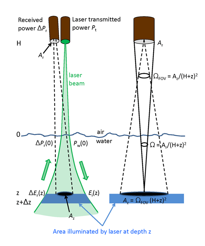
Figure 1 shows the geometry of the lidar system for detection of a scattering layer.

Figure 1: Geometry of the lidar system for detection of a scattering layer. The left panel illustrates the physical variables. The right panel illustrates the system optics; this panel ignores refraction at the sea surface.

The volume scattering function (VSF)

Recall from Eq. (1) of the Volume Scattering Function page that the volume scattering function (VSF) is operationally deﬁned by

β (ψ) = \frac{Δ Φ_{s} (ψ)}{Φ_{i} Δ z Ω},

where $Φ_{i}$ is the power incident onto an element of volume deﬁned by a surface area $A$ and thickness $Δ z$ , and $Δ Φ_{s} (ψ)$ is the power scattered through angle $ψ$ into solid angle $Ω$ . These quantities are illustrated in Fig. 2. In this derivation, quantities directly proportional to the layer thickness $Δ z$ will be labeled with a $Δ$ . Thus $Δ Φ_{s} (ψ)$ is the power scattered by the water layer of thickness $Δ z$ . The incident power $Φ_{i}$ onto area $A$ gives an incident irradiance $E_{i} = Φ_{i} ∕ A$ .

Figure 2: Quantities associated with the deﬁnition of the volume scattering function.

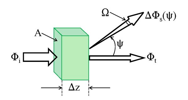
Now consider exact backscatter, which is a scattering angle of $ψ = π$ , or $ψ =$ 180 deg. The backscattered power $Δ Φ_{s} (π)$ exits the scattering volume through the same area $A$ , so the backscattered irradiance is $Δ E_{s} (π) = Δ Φ_{s} (π) ∕ A$ . The VSF for exact backscatter can then be written as

β_{π} \equiv β (ψ = π) = \frac{Δ Φ_{s} (π) ∕ A}{(Φ_{i} ∕ A) Δ z Ω} = \frac{Δ E_{s} (π)}{E_{i} Δ z Ω} .

This gives

Δ E_{s} (π) = E_{i} β_{π} Ω Δ z .

(1)

(Do not confuse this backscattered or reﬂected irradiance with $E_{u} = R E_{d}$ , which is deﬁned for any incident radiance distribution and for an arbitrarily thick layer of water. Here $E_{i}$ is the irradiance for a collimated incident laser beam and a thin layer of water.)

The beam spread function (BSF)

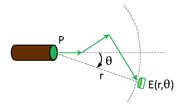
Suppose a collimated beam is emitting power $P$ in direction $𝜃 = 0$ . Then scattering and absorption in the medium will give some irradiance $E (r, 𝜃)$ on the surface of a sphere of radius $r$ at an angle of $𝜃$ relative to the direction of the emitted beam, as illustrated by the green arrow in Fig. 3. The beam spread function (BSF) is then deﬁned as

B S F (r, 𝜃) \equiv \frac{E (r, 𝜃)}{P} (m^{- 2}) .

(2)

Figure 3: Geometry for deﬁnition of the beam spread function.

The beam spread function and its equivalent, the point spread function, are discussed in more detail on the Beam and Point Spread Functions page.

Derivation of the Lidar Equation

The derivation of the lidar equation for the stated application now proceeds via the following steps:

1.

As illustrated in Fig. 1, the laser pulse has transmitted power

P_{t}

to start. After transmission through the atmosphere and sea surface, the pulse has power

P_{w} (0) = P_{t} T_{a} T_{s}

just below the water surface.

2.

The laser pulse is still a narrow beam when it enters the water, but it then begins to spread out because of scattering, and it is attenuated by absorption. This process is quantiﬁed by the beam spread function. We are interested in the “on-axis” irradiance incident onto a layer of water at depth

z

. From Eq. (2), this is given by

E_{i} (z) = P_{w} (0) B S F (z, 𝜃 = 0) .

3.

The irradiance that is reﬂected by a layer of thickness

Δ z

at depth

z

is given by Eq. (1):

Δ E_{r} (z) = E_{i} (z) β_{π} (z) Ω Δ z .

The solid angle $Ω$ is determined by the aperture size of the receiver and the distance from the receiver to the layer. This is discussed in step 7 below.

4.

The irradiance

Δ E_{r} (z)

heading upward from the layer

Δ z

will be attenuated by some diﬀuse attenuation function

{\bar{K}}_{u p}

Δ E_{r}

propagates back to the sea surface:

Δ E_{r} (0) = Δ E_{r} (z) exp (- {\bar{K}}_{u p} z) .

The receiver sees only an area $A_{z}$ depth depth $z$ . It is assumed that $A_{z}$ is less than the total area illuminated by the spreading laser beam at depth $z$ . Thus we can multiply $Δ E_{r} (z)$ by $A_{z}$ to get the power leaving the illuminated area that is seen by the receiver. The fraction of the total power reaching the surface, which is seen by the detector, is then

Δ P_{r} (0) = Δ E_{r} (z) A_{z} exp (- {\bar{K}}_{u p} z) .

$A_{z}$ is determined by the receiver ﬁeld of view and the distance from the receiver to the layer.

5.

The power just below the surface is now transmitted through the water surface and through the atmosphere to the receiver. The power detected is then

Δ P_{r} = Δ P_{r} (0) T_{s} T_{a} .

6.

Combining the above results gives

Δ P_{r} = P_{t} T_{a}^{2} T_{s}^{2} A_{z} Ω B S F (z, 0) β_{π} exp (- {\bar{K}}_{u p} z) Δ z .

7.

A_{z}

and

Ω

can be written in terms of known parameters. We are interested only in power that is reﬂected by the layer

Δ z

into the solid angle

Ω

that will take the light into the receiver. As shown in the right panel of Fig. 1, the receiver aperture

A_{r}

and the range

H + z

determine

Ω = A_{r} ∕ {(H + z)}^{2}

. Only power heading into

Ω

from area

A_{z}

, which is seen by the receiver, reaches the receiver.

A_{z}

is determined by the receiver ﬁeld of view solid angle

Ω_{F O V}

and the range:

A_{z} = Ω_{F O V} {(H + z)}^{2}

. Thus the

A_{z} Ω

factor in the preceding equation can be rewritten as

A_{z} Ω = Ω_{F O V} {(H + z)}^{2} \frac{A_{r}}{{(H + z)}^{2}} = A_{r} Ω_{F O V} .

This equation shows how the receiver optics aﬀects the detected power. (This is an application of the “ $A Ω$ ” theorem of optical engineering. $A Ω$ is also called the throughput or étendue of the system. Strictly speaking, the in-air solid angle $Ω_{F O V}$ decreases by a factor of $1 ∕ n^{2}$ upon entering the water, where $n$ is the water real index of refraction. However, the in-water $Ω$ increases by a factor of $n^{2}$ when entering the air. For a round trip, air to water to air, these $n^{2}$ factors cancel. They are thus ignored here and in Fig. 1.)

8.

Collecting the above results gives the desired lidar equation:

Δ P_{r} = P_{t} T_{a}^{2} T_{s}^{2} A_{r} Ω_{F O V} B S F (z, 0) β_{π} exp (- {\bar{K}}_{u p} z) Δ z .

(3)

Equation (3) nicely shows the eﬀects of the transmitted power ( $P_{t}$ ), atmospheric and surface transmission ( $T_{a}^{2} T_{s}^{2}$ ), receiver-optics ( $A_{r} Ω_{F O V}$ ), water-column ( $B S F (z, 0) β_{π} exp (- {\bar{K}}_{u p} z)$ ), and layer thickness ( $Δ z$ ). The take-home message from this equation is that in order to understand lidar data, the water inherent optical properties you need to know are the beam spread function and $β_{π}$ . This observation was in part the incentive for the work of Mertens and Replogle (1977), Voss and Chapin (1990), Voss (1991), McLean and Voss (1991), Maﬃone and Honey (1992), Gordon (1994b), McLean et al. (1998), Sanchez and McCormick (2002), Dolin (2013), Xu and Yue (2015), and others. These papers present several models for beam/point spread functions in terms of the water absorption and scattering properties. Several of those models are reviewed in Hou et al. (2008).

There are various arguments about what to use for ${\bar{K}}_{u p}$ , which depends on both the water optical properties and on the imaging system details. It is intuitively expected that ${\bar{K}}_{u p}$ , which is deﬁned for a horizontally small patch of upwelling irradiance, will be greater than the diﬀuse attenuation coeﬃcient for upwelling irradiance, $K_{u}$ , which is deﬁned for a horizontally inﬁnite light ﬁeld. Likewise, we expect that ${\bar{K}}_{u p}$ will be less than $c$ , the beam attenuation coeﬃcient. Thus $K_{u} < {\bar{K}}_{u p} < c$ . Because ${\bar{K}}_{u p}$ is an attenuation function for a ﬁnite patch of reﬂected irradiance, computing its value is inherently a three-dimensional radiative transfer problem. To pin down the value of ${\bar{K}}_{u p}$ more accurately thus requires either actual measurements for a particular system and water body, or three-dimensional raditative transfer simulations (usually Monte Carlo simulations) tailored to a given system and water properties.

Example calculation

To develop some intuition about Eq. (3), consider the following example application. Suppose a 532 nm laser is being used to look for objects in the water that have an area of $1 m^{2}$ . The receiver FOV must be small enough that the object can be distinguished from its surroundings. For $H = 100 m$ and $z = 10 m$ , this requires that

Ω_{F O V} \leq \frac{1 m^{2}}{(100 + 10) m^{2}} \approx 8 \times 1 0^{- 5} s r .

For a 15 cm radius receiving telescope, $A_{r} = π {(0.15 m)}^{2} \approx 0.07 m^{2}$ . For normal incidence at the sea surface, $T_{s} \approx 0.97$ , and for a clear atmosphere, $T_{a} \approx 0.98$ . Suppose the water is Jerlov type 1 coastal water for which $K_{d} (532) \approx 0.15 m^{- 1}$ (Light and Water, page 130), and assume that ${\bar{K}}_{u p} = K_{d}$ . Further assume that $B S F \approx exp (- 0.2 z)$ , since the lidar beam attenuation will be more “beam like” than diﬀuse attenuation, and $c > K_{d}$ . Finally, take $β_{π} = 1 0^{- 3} m^{- 1} s r^{- 1}$ (Light and Water, Table 3.10 for “coastal ocean” water). Then for $Δ z = 1 m$ at a depth of 10 m, the water returns the fraction

\begin{array}{l} \frac{Δ P_{r}}{P_{t}} = & {(0.98)}^{2} {(0.97)}^{2} (0.07) (8 \times 1 0^{- 5}) e^{- (0.2) 10} (1 0^{- 3}) e^{- (0.15) 10} (1) \\ \approx & 1.5 \times 1 0^{- 10} \end{array}

of the transmitted power.

Now suppose that the laser beam hits an object at $z$ = 10 m whose surface is a Lambertian reﬂector of 2% (irradiance) reﬂectance. Then 0.02 of $E_{i}$ is reﬂected into $2 π s r$ . The layer backscatter $β_{π} Δ z = 0.001 s r^{- 1}$ is then replaced by

\frac{0.02}{2 π s r} \approx 0.003 s r^{- 1} .

If all other terms remain the same, the object would return about three times the signal as the water itself.