Page updated:
March 22, 2021
Author: Curtis Mobley
View PDF
Spreading Function Effects
The last figure on the previous page shows a contour plot of a two-dimensional, one-sided variance spectrum and a contour plot of a random surface generated from that variance spectrum. A particular spreading function is implicitly contained in that two-dimensional variance spectrum. The effect on the generated sea surface of the spreading function contained within warrants discussion.
As we have seen (e.g. Eq. 4 of the Wave Variance Spectra: Examples page), a 2-D variance spectrum is usually partitioned as
Here is the omnidirectional spectrum, and is the nondimensional spreading function, which shows how waves of different frequencies propagate (or “spread out”) relative to the downwind direction at .
One commonly used family of spreading functions is given by the “cosine-2S” functions of Longuet-Higgins et al. (1963), which have the form
| (1) |
where is a spreading parameter that in general depends on , wind speed, and wave age. is a normalizing coefficient that gives
| (2) |
for all .
Figure 1 shows the cosine-2S spreading functions for values of and 20. These spreading functions are strongly asymmetric in , so that more variance (wave energy) is associated with downwind directions () than upwind (). The larger the value of , the more the waves propagate almost directly downwind (), rather than at large angles relative to the downwind direction. However, the cosine-2S spreading functions always have a least a tiny bit of energy propagating in upwind directions, as can be seen for the curves. This is crucial for the generation of time-dependent surfaces, as will be discussed on the next page.
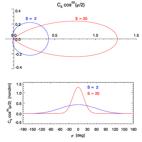
Figure 2 shows a surface generated with the omnidirectional variance spectrum of Elfouhaily et al. (1997) (ECKV) as used on the previous page, combined with a cosine-2S spreading function (1) with for all values. The wind speed is . The simulated region is using grid points. Note in this figure that the mean square slopes (mss) compare well with the corresponding Cox-Munk values shown in Table . The mss values for the generated surface are computed from finite differences, e.g.
averaged over all points of the 2-D surface grid. The and values shown in the figure are the average angles of the surface from the horizontal in the and directions). These are computed from
etc., averaged over all points of the surface.
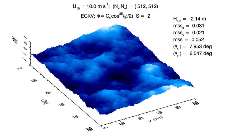
| slope variable | DFT value | Cox-Munk formula | Cox-Munk value |
| 0.031 | 0.032 | ||
| 0.021 | 0.019 | ||
| 0.052 | 0.054 | ||
The spreading function used in Fig 2 was chosen (with a bit of trial and error) to give a distribution of along-wind and cross-wind slopes in close agreement with the Cox-Munk values (except for a small amount of Monte-Carlo noise). Figure 3 shows a surface generated with a cosine-2S spreading function with ; all other parameters were the same as for Fig. 2. This value gives wave propagation that is much more strongly in the downwind direction , as would be expected for long-wavelength gravity waves in a mature wave field. The surface waves thus have a visually more “linear” pattern, whereas the waves of Fig. 2 appear more “lumpy” because waves are propagating in a wider range of angles from the downwind.
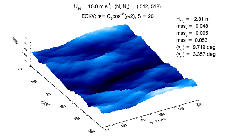
As shown in on the Wave Variance Spectra: Theory page , the total mean square slope depends only on the omnidirectional spectrum . Thus the total mss is the same (except for Monte Carlo noise) in both figures 2 and 3, but most of the total slope is in the along-wind direction in Fig. 3.
Real spreading functions are more complicated than the cosine-2S functions used here. In particular, some observations Heron (2006) of long-wave gravity waves tend to show a bimodal spreading about the downwind direction, which transitions to a more isotropic, unimodal spreading at shorter wavelengths. Although omnidirectional wave spectra are well grounded in observations, the choice of a spreading function is still something of a black art. You are free to choose any so long as it satisfies the normalization condition (2).
 See comments posted for this page and leave your own.