Terminology

Remote sensing, like any field of science, has specialized terminology, which we introduce here.

Active versus Passive Remote Sensing

Remote sensing can be active or passive.

Active remote sensing means that a signal of known characteristics is sent from the sensor platform—an aircraft or satellite—to the ocean, and the return signal is then detected after a time delay determined by the distance from the platform to the ocean and by the speed of light. One example of active remote sensing at visible wavelengths is the use of laser-induced fluorescence to detect chlorophyll, yellow matter, or pollutants. In laser fluorosensing, a pulse of UV light is sent to the ocean surface, and the spectral character and strength of the induced fluorescence at UV and visible wavelengths gives information about the location, type and concentration of fluorescing substances in the water body. Another example of active remote sensing is lidar bathymetry. This refers to the use of pulsed lasers to send a beam of short duration, typically about an nanosecond, toward the ocean. The laser light reflected from the sea surface and then slightly later from the bottom is used to deduce the bottom depth. The depth is simply $0.5\left(c∕n\right)\Delta t$, where $c$ is the speed of light in vacuo, $n$ is the water index of refraction, $\Delta t$ is the time between the arrival of the surface-reflected light and the light reflected by the bottom, and the 0.5 accounts for the light traveling from the surface to the bottom and back to the surface. Laser fluorosensing and lidar bathymetry are discussed in detail in Measures (1992) and on the page on The Lidar Equation.

Passive remote sensing simply observes the light that is naturally emitted or reflected by the water body. The night-time detection of bioluminescence from aircraft is an example of the use of emitted light at visible wavelengths. The most common example of passive remote sensing, and the one primarily discussed in this chapter, is the use of sunlight that has been scattered upward within the water and returned to the sensor. This light can be used to deduce the concentrations of chlorophyll, CDOM, or mineral particles within the near-surface water; the bottom depth and type in shallow waters; and other ecosystem information such as net primary production, phytoplankton functional groups, or phytoplankton physiological state.

Data Resolution

The quality of remote sensing data is determined by the spatial, spectral, radiometric and temporal resolutions.

• Spatial resolution refers to the “ground” size of an image pixel, which may be as small as 1 m for airborne systems to more than 1000 meters for satellite systems.
• Spectral resolution refers to the number, spacing, and width of the different wavelength bands recorded. This can range from one broad band covering the visible spectrum to several hundred bands, each a few nanometers wide. The spectral resolution is quantified by the
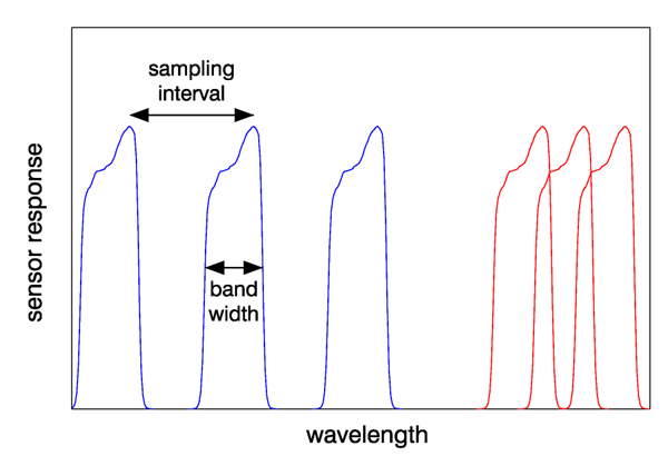
  • Sampling interval, which is the spectral distance between the centers or peaks of adjacent spectral channels along a spectrum
  • Band width (or band pass), which is the full width at half maximum (FWHM) of a spectral channel response to monochromatic light

  Figure 1 illustrates the difference in sampling interval and band width. The three blue curves indicate a sampling interval that is greater than the band width, as is common for multispectral sensors. The red curves illustrate a sampling interval that is less than the band width, which is often the case for hyperspectral sensors.

  ---

  
  

  Figure 1: Illustration of the difference in sampling interval and band width.

  ---

  Spectral resolution can be further described the sensor type:

  • Monochromatic refers to a sensor with 1 very narrow wavelength band, e.g. at a laser wavelength.
  • Panchromatic refers to 1 very broad wavelength band, usually over the visible range, e.g. a black and white photograph.
  • Multispectral sensors have several (typically 5-10) wavelength bands, each typically 10-20 nm wide.
  • Hyperspectral sensors have 30 or more bands with 10 nm or better resolution. Typical hyperspectral sensors have more than 100 bands, each less than 5 nm wide.
• Radiometric resolution refers to the number of different intensities of light the sensor is able to distinguish, often specified as the number of recorded bits. An n-bit sensor can record $2^n$ levels of light intensity between the smallest or darkest expected value (usually zero, or no light) and the brightest expected value. Typically sensors range from 8 to 14 bits, corresponding to $2^8=256$ to $2^{14}=16,384$ levels or “shades” of color in each band. The radiometric resolution determines how small of a change in the measured quantity can be recorded by the instrument. Usable resolution depends on the instrument noise.
• Temporal resolution refers to the frequency of flyovers by the sensor. This is relevant for time-series studies, or if cloud cover over a given area makes it necessary to repeat the data collection.

Data processing levels

Processing remotely sensed imagery involves many steps to convert the radiance measured by the sensor to the information desired by the user. These processing steps result in different “levels” of processed data, which are often described as follows:

• Level 0 refers to unprocessed instrument data at full resolution. Data are in ”engineering units” such as volts or digital counts.
• Level 1a is unprocessed instrument data at full resolution, but with information such as radiometric and geometric calibration coefficients and georeferencing parameters appended, but not yet applied, to the Level 0 data.
• Level 1b data are Level 1a data that have been processed to sensor units (e.g., radiance units) via application of the calibration coefficients. Level 0 data are not recoverable from level 1b data. Science starts with Level 1b data.

  Atmospheric correction converts the top-of-the-atmosphere radiance of Level 1b to normalzed water-leaving reflectance ${\left[\rho \right]}_N^{ex}$ of Level 2. ${\left[\rho \right]}_N^{ex}$ is defined on the Normalized Reflectances page.

• Level 2 refers to normalzed reflectance ${\left[\rho \right]}_N^{ex}$ and derived geophysical variables (e.g., chlorophyll concentration or bottom depth) at the same resolution and location as Level 1 data.
• Level 3 are variables mapped onto uniform space-time grids, often with missing points interpolated or masked, and with regions mosaiced together from multiple orbits to create large-scale maps, e.g. of the entire earth.
• Level 4 refers to results obtained from a combination of satellite data and model output (e.g., the output from an ocean ecosystem model), or results from analyses of lower level data (i.e., variables that are not measured by the instruments but instead are derived from those measurements).

Validation

It is always of interest to compare remotely sensed values with “ground truth” or known values, usually measured in situ, of the quantity being determined by remote sensing. This leads to various ways of describing the difference in remotely sensed and in situ values of the same quantity.

• Reliability refers to the certainty with which the value of a remotely sensed quantity is actually a measure of the quantity of interest. For example, if chlorophyll concentration is the quantity of interest, it is desirable that the value obtained be a measure only of chlorophyll and not, perhaps, a false value caused by high concentrations of mineral particles or dissolved substances that can change a spectrum so as to give an incorrect chlorophyll value in a retrieval algorithm. A reliable cholorphyll retrieval algorithm would give the chlorophyll value regardless of what other substances are in the water. (Note that in some fields, reliability is defined as the ability to reproduce a measurement; this is different that the meaning used here.)
• Reference value is the quantity (often measured in situ) being used for comparison with a remotely sensed value. This is often thought of as the “true” value of the quantity, but it must be remembered that the “truth” is seldom known. A value measured in situ is also subject to errors determined by the instrument and methodology used, and thus also may not be the true value of the quantity being measured.
• Error is the difference between a measurement and a reference value. Errors can be systematic or random.
  • Random errors are differences between a measurement and a reference value that are determined by random physical processes such as electronic noise. Although the statistical properties of the errors can be determined, the value of the error in any particular measurement cannot be predicted. The statistical distribution of random errors is often assumed to be Gaussian, but this is often just a mathematical convenience rather than a correct description of the underlying physical process. The effects of random errors can be reduced by making repeated measurements of the same quantity and then averaging the results.
  • Systematic errors are biases or offsets between a measurement and reference value that are caused by imperfect instruments, methodologies, or algorithms. Examples are additive offsets caused by failure to remove dark current values or multiplicative errors caused by imperfect instrument calibration. The purpose of instrument calibration is the removal of systematic errors from the measurements. The systematic error is quantified as the difference in the reference value and the average of repeated measurements. Systematic errors cannot be reduced by making additional measurements and averaging the results.
• Precision is the reliability with with an instrument will give the same value when repeated measurements of the same quantity are made. Precision is determined by repeated measurements, without regard for any reference value. It can be quantified by the standard deviation of the values measured.

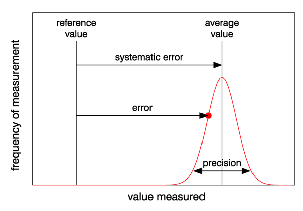
Figure 2 illustrates the differences in accuracy and precision, and systematic and random errors. The red curve represents the distribution of values obtained by many repeated measurements; the red dot represents any one of those measurements. The arrow showing the precision is drawn as the mean value $\pm 1.96$ standard deviations of the measured values; this means that 95% of the measurements lie within that range of values. In this example, there is a large systematic error, so that the measured quantity is not very accurate, but there is a relatively small spread of measured values, so that the precision is high compared to the systematic error. Ideally, measurements have a small systematic error and high precision. In practice, if repeated measurements can be made, it is better to have a small systematic error even if the precision is low, because averaging repeated measurements reduces the effects of random errors and leads to an accurate average value.

Finally, when developing a mathematical model or algorithm, there are two potential sources of error. The model may leave out some of the physical processes essential to describing the phenomenon of interest. Even if the physics is correct, there may be errors in the computer programming of the model equations. The model must be checked for both of these types of errors.

• Verification refers to making sure that the model equations have been programmed correctly.
• Validation then refers to checking the model output against reference values to make sure that both the model physics and the computer programming are correct.