Polarization: Stokes Vectors

What is Polarization?

Light consists of propagating electric and magnetic fields, which are described by Maxwell’s equations. If the time- and space-dependent electric field vector $E\left(x,t\right)$ is known, then the magnetic field vector $B\left(x,t\right)$ can be computed from Maxwell’s equations, and vice versa. It is thus sufficient to discuss just one of these fields, which is customarily chosen to be the electric field vector. Polarization then refers to the plane in which the electric field vector is oscillating.

Suppose you are looking toward a light source, or “into the beam.” In the simplest case, called linear (or plane) polarization, the electric field $E\left(x,t\right)$ lies in, or oscillates in, a fixed plane. The animation below illustrates how the electric field varies with time as the light wave passes through a fixed reference plane normal to the direction of propagation. (Animation from https://en.wikipedia.org/wiki/Polarization_(waves)) For visible wavelengths, these oscillations are at a frequency of around $10^{14}$ times per second and cannot be directly measured because of instrumentation limits.

However, the plane in which the electric field lies may also rotate with time as the beam of light passes. This is called circular polarization if the maximum value of $E\left(x,t\right)$ is independent of time but the orientation of the plane rotates. There is an intermediate state, elliptical polarization, in which the plane rotates and the amplitude of $E\left(x,t\right)$ also changes as the plane rotates, so that the maximum value of $E\left(x,t\right)$ traces out an ellipse. The final possibility is that, as you observe $E\left(x,t\right)$, the plane of oscillation changes rapidly (on the order of the frequency of the light) and randomly. This is random polarization, which is often called “unpolarized” or “natural” light.

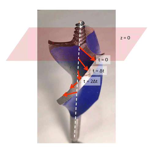
Circular or elliptical polarization is called “right” or “left” depending on the direction the plane of the electric field rotates as the wave passes a fixed reference plane, but understanding the exact meaning these terms as they relate to light can be confusing. Figure 1 makes an analogy to a common “right-hand-twist” drill bit used to cut holes in wood. The edges of this bit form right-handed helices as commonly defined. As this bit bores into the wood, the cutting tips trace out right-handed helices. Now think of the outer edge of the bit as being the tip of the electric field vector of circularly polarized light. The light is propagating upward in the figure, in the direction the drill goes into the wood. The reddish plane labeled $z=0$ is held fixed in space as the light propagates past this reference plane. The red arrow labeled $t=0$ indicates the electric field vector lying in the reference plane at time zero. Now think of moving the drill bit upward without rotating it. At some time $t=\Delta t>0$ later the drill bit/light wave will have moved upward, and the red arrow labeled $t=\Delta t$ will lie in the reference plane. The $t=\Delta t$ vector will have rotated from the direction of the $t=0$ vector. At time $t=2\Delta t$ the light wave will have moved further upward, and the $t=2\Delta t$ vector will now be crossing the reference plane at $z=0$. As time progresses, the direction of the electric field vectors in the reference plane will appear to rotate in a clockwise direction as viewed looking into the beam (or counterclockwise when looking along the beam). This is the electric field rotation direction for right-circularly polarized (RCP) light. If the electric field rotates in a counterclockwise direction when looking into the beam (or clockwise looking along the beam), the light is left-circularly polarized (LCP).

Note that the description of the electric field as rotating clockwise or counterclockwise depends on whether you are looking into the beam or along the beam. However, the concept of right-handed vs. left-handed helices is independent of the viewing perspective. The definition just described—RCP corresponds to clockwise electric field rotation in a reference plane when looking into the beam as the light propagates through the plane, and to the pattern of electric field vectors lying along a right-hand helix in space—is what is used by Bohren and Huffman (1983) and Hecht (1987). I personally like that convention because I can remember the analogy with the moving right-hand-helix drill bit. However, others (e.g., Kattawar (1994) and Jackson (1962)) use the opposite convention of RCP meaning that the electric field appears to rotate counterclockwise with looking into the beam (or clockwise looking along the beam); in this choice LCP corresponds to a right-handed helix. The convention for how to define RCP vs LCP often seems to depend on the field of the user—physics vs. astronomy vs. chemistry, etc. Fortunately it does not matter which one you use, so long as you make a choice and stick with it during the solution of your problem. Problems arise only if you compare your results with someone else’s results, in which case different descriptors like parallel vs. perpendicular and right vs. left may be referring to the same thing by different names.

The animation below (from https://en.wikipedia.org/wiki/Circular_polarization shows the propagating electric field of RCP light as defined here, but that page calls it LCP, which was the choice for the creator of that Wikipedia page.

Stokes Vectors

We now need a quantitative way to specify the state of polarization of light. This is given by the Stokes vector, which is an array of four real numbers usually written as

Note that $\underline{S}$ is just an array with four elements; it is not a vector in the geometric sense.

To define the Stokes vector, first pick an $\left(\widehat{x},ŷ,ẑ\right)$ coordinate system that is convenient for your problem. In a laboratory setting, this system might have $\widehat{x}$ parallel to an optical bench top, $ŷ$ perpendicular to the bench top, and $ẑ=\widehat{x}\times ŷ$ in the direction of propagation. In this lab setting, $\widehat{x}$ might then be called the “parallel” (to the bench top) direction, and $ŷ$ would then be the “perpendicular” direction. Or $\widehat{x}$ and $ŷ$ might be called “horizontal” and “vertical”, respectively. The Level 2 page on scattering of polarized light shows another coordinate system commonly used in oceanography.

The electric field vector in this coordinate system is resolved into x and y components as $E=E_x\widehat{x}+E_yŷ$, where the components $E_x$ and $E_y$ depend on position and time. For light propagating in a vacuum, the electric field is transverse to the direction of travel, so the z component of $E$ is zero. If the light is linearly polarized in the x plane, then $E_x\ne 0$ and $E_y=0$. For linear polarization in the y plane, $E_x=0$ and $E_y\ne 0$.

At optical frequencies we cannot measure instantaneous value of the fluctuating electric field $E\left(t\right)$ itself, but we can make time-averaged (over many wave periods) measurements of the corresponding irradiance $\mathcal{ℰ}$. The time-averaged irradiance corresponding to $E\left(z,t\right)=E_{o}exp\left(ikz-i\omega t\right)$ is

Here ${𝜖}_m$ is the electrical permittivity of the medium, which has units of $Farad{m}^{-1}$ or $C^2{N}^{-1}{m}^{-2}$ or $A^2{s}^{4}k{g}^{-1}{m}^{-3}$. ${\mu }_m$ is the magnetic permeability of the medium, which has units of $Henry{m}^{-1}$ or $N{A}^{-2}$ or $kgm{s}^{-2}{A}^{-2}$. Electric fields have units of $N{C}^{-1}$ or $V{m}^{-1}$ or $kgm{s}^{-2}{C}^{-1}$. Thus $\mathcal{ℰ}$ has units of $kg{s}^{-3}$ or $Watt{m}^{-2}$, i.e. of irradiance. The factor of $\frac{1}{2}$ comes from the average of the sinusoidal dependence of $|E\left(t\right){|}^2$ over a wave period (i.e., $\frac{1}{2\pi }{\int \; <!--nolimits-->}_0^{2\pi }{cos}^{2}xdx=\frac{1}{2}$). We therefore base the definition and actual measurements of Stokes vectors on the measurable time-averaged irradiances if we are working with a collimated monochromatic beam of light.

The $Q$ Stokes parameters is then defined follows. Let ${\mathcal{ℰ}}_x$ be the time averaged irradiance measured with a linear polarizing filter placed in the beam and oriented in the x (or parallel or horizontal in the lab setting) direction. Let ${\mathcal{ℰ}}_y$ be the time average measured with the linear polarizer oriented in the y (or perpendicular or vertical) direction. Then $Q$ is defined as

Thus $Q>0$ if the polarization lies in the x plane, and $Q<0$ if it lies in the y plane.

This choice of $\widehat{x}$ and $ŷ$ can distinguish between linear polarization lying in the x or y planes. But suppose that the plane of polarization is intermediate between the x or y planes, as illustrated by the either of the red arrows in the left panel of Fig. 2. These are different states of polarization, but both have the same projections onto the x and y planes, hence the same $Q$ value. Thus the $Q$ parameter cannot distinguish between the solid and dashed planes of polarization seen in the left panel of the figure.

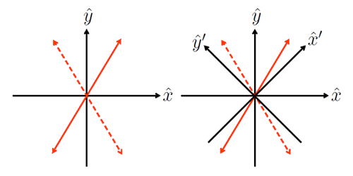
The state of linear polarization can be uniquely specified by the choice of a second set of axes, $\left({\widehat{x}}^{\prime },{ŷ}^{\prime }\right)$, chosen at a 45 deg angle to the $\left(\widehat{x},ŷ\right)$ axes, as shown in the right panel of Fig. 2. The solid and dashed red arrows have different projections on the $\left({\widehat{x}}^{\prime },{ŷ}^{\prime }\right)$ axes and are thus distinguished. The Stokes $U$ parameter is non-zero for planes of polarization like the red arrows in the figures and is defined by

where ${\mathcal{ℰ}}_{x^{\prime }}$ and ${\mathcal{ℰ}}_{y^{\prime }}$ are the time averages of the irradiances measured with the linear polarizer oriented in the $x^{\prime }$ and $y^{\prime }$ planes. Thus if the plane of polarization lies at 45 deg to the x plane, parallel to ${\widehat{x}}^{\prime }$, $U>0$ and $Q=0$. For polarization in the plane at -45 deg to the x plane, parallel to ${ŷ}^{\prime }$, $U<0$ and $Q=0$. For planes of linear polarization not lying in either the x,y or $x^{\prime },y^{\prime }$ planes (as illustrated by the red arrows in Fig. 2), both $Q$ and $U$ will be non-zero and either positive or negative, depending on the inclination of the polarization plane to these two sets of axes.

The Stokes parameters $Q$ and $U$ together specify the state of polarization if the light is linearly polarized. Another parameter, $V$, is needed to specify the state of circular polarization. The time-averaged amounts of right and left circularly polarized irradiance, call them ${\mathcal{ℰ}}_R$ and ${\mathcal{ℰ}}_L$ respectively, can be measured by use of circular polarizers. The $V$ component is then defined as their difference:

Thus $V>0$ for right circular polarization, and $V<0$ for left circular polarization.

Finally, consider the case of randomly polarized light. All of the above time averages will be equal because of the rapid fluctuations of the electric fields with all directions and helicities, in which case $Q=U=V=0$. To account for this case, let $I$ be the total irradiance without regard for the state of polarization. This is measured without the use of any polarization filters in the beam. This is also given in terms of the time averages by

$I$ is always positive and equal to the total irradiance.

It is important to note that the values of the $Q$ and $U$ parameters depend on the choice of the $\left(\widehat{x},ŷ\right)$ axes, but the values of $I$ and $V$ are independent of this choice. In the coordinate system described above, the $\widehat{x}$ axis is parallel to the horizontal laboratory bench top, and $ŷ$ is perpendicular to the bench top. As noted, it is common to refer to the corresponding polarizations as being “parallel” or “horizontal” and “perpendicular” or “vertica”, respectively. Terms like parallel and perpendicular or horizontal and vertical always refer to some reference plane—the bench top in this case. However, a different choice of the reference plane changes the meaning of these terms. One person’s parallel polarization can be another person’s perpendicular polarization. You have to figure out the meanings on a case by case basis for whatever reference coordinate system is being used.

If the beam is perfectly polarized (in whatever state of polarization), then

If the beam is unpolarized, or is a mixture of polarized and unpolarized light, then this relation becomes an inequality:

The degree of polarization, expressed in percent, is defined by

The degree of linear polarization is defined by

and the degree of circular polarization is defined by

DoCP is positive for RCP and negative for LCP. These measures of the degree of polarization do not depend on the choice of coordinate system.

The definitions of $Q,U$, and $V$ above were made in terms of measurable irradiances. There is much more that can be said, in particular about the theoretical formulation of the Stokes vector in terms of the solution of Maxwell’s equations for a propagating wave. An excellent and entertaining presentation of those details is given in Chapter 7 of Bohren and Clothiaux (2006). Suffice it to say that in discussions of Stokes vectors you may see them defined by equations such as

The first form of definition is in terms of irradiances as discussed above, with an obvious change in notation to show the orientations of the polarizing filters in the chosen coordinate system. The second form is written in terms of the complex, time-dependent, electric field vectors after describing the light beam in terms of a plane-wave solution to Maxwell’s equations. Thus $E_{\parallel }\left(t\right)=E_{o\parallel }exp\left(-i\omega t\right)$, etc. The $⟨...⟩$ notation indicates the time average of the argument. After the time averages are taken, the magnitudes $E_{o\parallel }$ etc. are left, and there is an additional factor of $\frac{1}{2}$ resulting from the average of products of the sinusoidal electric fields over a wave period. The final form makes clear that the Stokes parametes are real numbers. The discussion of Eq. (1) shows that the definitions in terms of electric fields still have units of irradiance. The irradiance form is what you will use in the lab; the electric-field forms are what you will use for theory.

Table 1 shows the pattern of Stokes parameters for various states of polarization.