Page updated:
March 13, 2021
Author: Curtis Mobley
View PDF
Particle Size Distributions
Figure 1 of the Introduction page of this chapter shows the size ranges commonly associated with different components of natural waters. This page discusses the theory of how to quantify the number of particles as a function of their size. The Level 3 page Creating Particle Size Distributions from Data discusses the mechanics of creating particle size distributions from measured data.
Non-uniqueness of Particle Size
The first problem is to decide what is meant by particle “size,” especially when speaking of statistical measures like the “average size” of a collection of particles.
Suppose we have three spherical particles of radii , and 3. What is the “average size” of these three spheres?
If the average size is based on the radius, then the average (radius) sphere has a radius of (1 + 2 + 3)/3 = 2.
If the average is based on the surface area of the spheres, , then the average surface area is which corresponds to a radius of . The same holds true for the cross-sectional area of the spheres.
If the average is based on the volume of the spheres, , then the average volume is which corresponds to a radius of .
So there is ambiguity in how to define the “average particle size” even for a collection of spherical particles.
The situation is ever worse for non-spherical particles, which do not have a single parameter like radius that can be used to specify the size of the particle. The “size“ of a non-spherical particle is sometimes taken to be
- the largest dimension of the particle,
- the arithmetic mean of the largest dimension of the particle, , and the smallest dimension, : ,
- the geometric mean of the largest and the smallest dimensions: ,
- the diameter of a sphere with the same surface area as the particle (an “area-equivalent” sphere), or
- the diameter of a sphere with the same volume as the particle (a “volume-equivalent” sphere),
and there are also other measures of the “size” of a non-spherical particle. Note that the arithmetic and geometric means are equal for spherical particles, but are in general not equal.
All of these measures of particle size are valid, but one measure may be optimum for a particular application. For example, a Coulter Counter measures the change in electrical conductivity when a particle passes through the sensor. This change is proportional to the amount of material in the particle, i.e. to the particle volume. Thus a Coulter Counter measures the the size of a volume-equivalent sphere. Laser diffraction instruments measure diffraction of light caused by a particle in the light beam. The angular shape of the diffraction pattern is determined by the cross-sectional (projected) area of the particle as seen by the beam. Thus laser diffraction measures the size of an area-equivalent sphere.
The diameters of area-equivalent and volume-equivalent spheres can be considerably different. Consider a cubical particle of length on a side. The volume is and the equivalent-volume sphere () has a diameter
The surface area of the cube is and of a sphere is , which leads to
If cubes of this size are seen randomly oriented in a laser beam, the average projected area is one-fourth of the surface area (Cauchy’s Average Projected Area Theorem, which shows that for a convex polyhedron, the average projected area over all orientations, i.e. the average cross section, is one-fourth the surface area of the polyhedron). Thus the laser sees, on average, particles of area , and the equivalent-projected-area sphere has diameter . This again leads to .
Thus for a cube the diameter of the equivalent-area sphere is 1.11 times the diameter of the equivalent-volume sphere. Coulter-principle and laser-diffraction instruments will therefore report somewhat different equivalent-sphere sizes for the same particle. Clearly, it is important to understand exactly what an instrument measures and what instrument was used to measure particle sizes.
Unfortunately, publications sometimes fail to state exactly what measure they are using for the size of non-spherical particles.
Particle Size Distributions
First decide on some measure of particle size; call it the diameter . If the particles are known to be spherical (e.g., fog droplets or small bubbles in water), then is the diameter of the sphere. For non-spherical particles, is most often taken to be the diameter of the volume-equivalent sphere. The next step is to quantify how many particles there are of each size . There are two equivalent ways to do this.
The cumulative number size distribution () is usually defined (in the particle-sizing literature) as the number of particles per unit volume larger than size . is usually expressed in units of . In principle, this function can be measured simply by counting the numbers of particles larger than a given size , as in principle ranges from 0 to , but in practice ranges from some minimum to some maximum . These minimum and maximum sizes are usually determined by the instrument used to do the counting.
The particle number size distribution () is a function defined so that is the number of particles per unit volume between size and (or in the size range ). The units of are usually number of particles per cubic meter per micrometer of size range, i.e. .
The , , as defined above decreases as increases, so is negative. The corresponding PSD is then the negative of the derivative of the CSD, and is usually written as
| (1) |
Because of the large range of values for both and , it is customary to plot these functions on log-log scales and to work with logarithmic size intervals. You then see (e.g., Junge (1953) and Liley (1992)) defined in terms of a log derivative, which is related to by
| (2) |
The comes from a change of base from base 10 logarithms, which are convenient for working with data, to base natural logarithms, which are convenient for mathematics. Thus PSDs defined by logarithmic and linear derivatives will differ by a factor of :
The converse of Eq. (1) is
The total number of particles per unit volume is given by
In the particle sizing literature, it is customary to use a diameter as the measure of particle size. However, Mie Theory usually expresses its size parameter in terms of the particle radius . If using a PSD(D) in Mie calculations as described on the Mie Theory page, it is necessary to use .
Area and volume size distributions
The previous definition (1) of the PSD was for the number of particles in a unit volume, hence the notation or , with the subscript indicating number of particles, and the name number size distribution. We can also define size distributions for the area and volume of the same particles. The surface area of a sphere is , so the PSD for area (subscript ) is
| (3) |
Note that the units of the area size distribution are particle surface area, usually in , per unit volume per unit size interval. The size distribution for the cross-sectional area of the particles is , with the same units. The PSD for particle volume, , is then (subscript )
| (4) |
Now the units of the volume size distribution are particle volume, usually in units of , per unit volume per unit size interval. For particle volume measured in cubic micrometers, thus gives a size distribution for particle volume in parts per million, per unit size interval. Of course, these formulas are based on the assumed validity of area- and volume-equivalent spheres.
The total surface area of particles per unit volume is
The total volume of particles per unit volume is
If the quantity of interest is the number of particles (e.g., the number of phytoplankton of various sizes), then the number size distribution is the relevant distribution. However, some processes depend more on the surface area of the particles than on their number. For example, chemical reactions such as combustion (e.g., burning of coal dust in a power plant) depend strongly on the surface area, and laser diffraction is governed primarily by particle cross-sectional area. For such problems, is the distribution of interest. For processes that depend on particle volume or mass (e.g., the mass of sediment material resuspended in a bottom boundary layer or particle buoyancy in a fluid), the volume distribution is the distribution of interest.
Many commercial particle sizing instruments allow the user to select the output as a number, area, or volume PSD. Keep in mind that the conversions between one form of PSD and another are being made on the basis of an assumed equivalent spherical particle, even though the underlying measurement may be based on particle area (laser diffraction) or volume (Coulter counter). Thus a laser diffraction instrument may give a good measurement for the area even for nonspherical particles, but errors can be introduced when converting the area PSD to number or volume PSDs. A Coulter counter may give a good measurement of a volume distribution even for nonspherical particles, but errors can be introduced with converting the volume distribution to area or number distributions.
Comments on terminology
As is so often the case, different authors sometime use different terminology. For example, Bader (1970) calls the cumulative number distribution function and the number distribution function. Jonasz (1983) calls the cumulative size distribution and the particle size distribution. I use the term cumulative number size distribution () for and particle number size distribution () for because that seems to be the most common in the literature (subscript for number).
However, in probability theory, a cumulative distribution function refers to the how much of a total is less than , rather that greater than as used for . Runyan et al. (2020) compute a true by dividing the by the total number of particles over all sizes, , to get a true , and then computing a (nondimensional) CDF as . They also employ a carefully designed nomenclature with , , and denoting the number, area, and volume PDFs, which they refer to as density functions. This is somewhat in analogy to a spectral density function, which shows how much of something there is per unit interval of distance or frequency. Their true CDFs are denoted by , and for the number, area, and volume CDFs computed from the respective density functions.
Any of the functions ), , , , ), , etc. is properly termed a particle size distribution. They are all different ways of describing how some feature of particles (number, area, volume) change with size, and one can be computed from and of the others (under certain assumptions like spherical particle shapes).
I suspect that the “backwards” definition of the cumulative size distribution as used in particle analysis traces back to measurement of size distributions of soil or other particles using a succession of wire mesh sieves. You first sieve out the large particles (gravel, for example) and count those. Then a smaller mesh collects the next smaller size (sand, for example), and so on down to the finest particles (e.g., silt). The fine meshes are very delicate, so you have to remove the large particles first. Thus as the sieving process works from large to small particles sizes, you are accumulating the number of particles larger than the current sieve size, and building up a that shows how many particles are larger than . Given a normalized probability distribution function (e.g, , it is convenient to integrate (or sum) the PDF from small to large values of , and thus build up a that shows the fraction of the total that is less than .
Models for Particle Size Distributions
Many models have been proposed for particle size distributions. These differ according to the environment (atmosphere, ocean, industrial process) and particular data set being analyzed. The classic studies by Junge (Junge (1953), Junge (1955)) were concerned with aerosol size distributions. He found that a number size distribution of the form
| (5) |
gave a good fit to aerosols down to about in diameter. Note that according to Eq. (2), the dependence of Eq. (5) corresponds to a dependence when written as
| (6) |
Thus you usually see the statement than a Junge distribution has a slope of -4 when and are plotted on logarithmic axes.
Figure 1 shows one instance of the number PSD for various size classes of marine biological particles; is the diameter of a volume-equivalent sphere. The Junge distribution is shown as a blue line, with the magnitude fixed by the value for picoplankton.
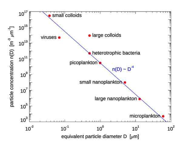
A more general number size distribution model is the power law distribution, which is usually written as
| (7) |
The exponent is usually called the slope parameter. is the value of the distribution in at a reference diameter . The Junge distribution (6) is a special case of a power law distribution for . (Some authors call the power law distribution a Junge distribution, but others are careful to use the term Junge distribution only for because that is the only slope Junge considered in his papers.)
Figure 2 shows 168 number size distributions measured over the equivalent-sphere size range in Arctic waters. When fit to the power law model of Eq. (7), the best-fit values of have the distribution of values shown in Fig. 3. The average of the 168 slope parameters is .
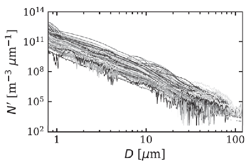
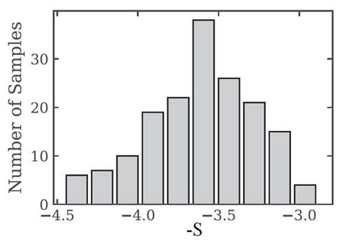
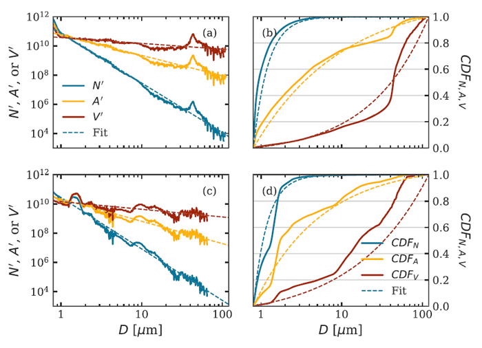
Figure 4 shows two of the PSDs of Fig. 2 along with the corresponding area and volume distributions, and the cumulative distribution functions. Although the fit of the power-law model (7) to these number PSDs appears quite good on a log-log plot, it must be noted that there are order-of-magnitude deviations from the best-fit curves, namely near - in the upper left figure, and near in the lower-left figure. Such deviations are common in fits such as these and can result, for example, from a bloom of a particular species of phytoplankton. It should be noted from the CDFs in the right panels that the total number of particles comes mostly from particles less than about , but the total volume of particles comes mostly from the larger particles greater than about . This is simply because one particle with has as much volume as 1000 particles of size , for example.
It sometimes happens that the small size and large size ends of the distribution have different slopes. A better fit is then obtained by separate fits of a power law for the two size regions, but other distributions have also been used.
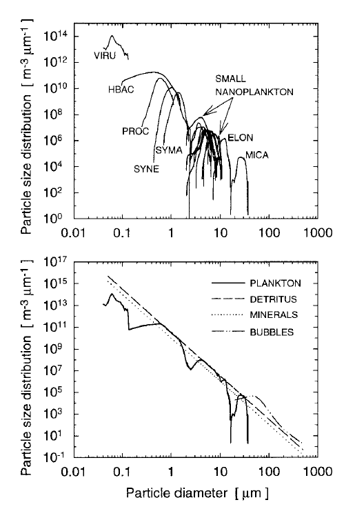
It is important to recognize that a power-law distribution implies that the size range extends from to . This is never the case in nature. The smallest phytoplankton have a diameter of about and the largest are about . Thus a PSD for phytoplankton, whatever its mathematical form, should be applied only for the to size range, and perhaps for an even smaller range. Particular species or size classes of phytoplankton have much small size ranges. The upper panel of Fig. 5 shows measured number PSDs for 18 classes and species of phytoplankton (VIRU is viruses, HBAC is heterotrophic bacteria, PROC is prochlorococcus, ..., MICA is Prorocentrum micans; see Stramski et al. (2001) for the full listing and description of these microbes). The bottom panel of the figure show the sum of the individual PSDs, with the concentrations of each class chosen within the ranges of typical values so that the total (except for viruses) obeys a Junge distribution ( in Eq. (7)). Modeled distributions for detritus, minerals, and bubbles are also shown. These PSDs were used to model the inherent optical properties of oligotrophic waters; the total chlorophyll of the sum is .
The PSDs of individual species or classes of particles as seen in the upper panel of Fig. 5 are often modeled by a log-normal distribution. In this distribution, the numbers are normally distributed when is plotted on a logarithmic scale as in the preceding figures, or equivalently, using a normal distribution in rather than in . That is, is distributed as a Gaussian probability distribution function:
| (8) |
where and are the mean and standard deviation of , respectively. Note that this satisfies
as is required of any probability distribution function. Noting that represents the same probabilities gives
which is the form seen in Eq. (A1) of Campbell (1995), and is equivalent to Eq. (2) of Ahmad et al. (2010). To express the log-normal distribution in terms of base 10 logarithms, the same procedure plus the observation that gives
which is the form seen in Eq. (1) of Shettle and Fenn (1979). Now and are the mean and variance of . (Note that is defined for , which corresponds to in Eq. (8).) Multiplying these probability distribution functions by magnitudes (e.g., the total number of particles per cubic meter) scales them for use as PSDs.
Log-normal distributions are commonly used to describe atmospheric aerosol size distributions (e.g., Shettle and Fenn (1979)). The current NASA atmospheric correction algorithm models aerosols as a sum of two log-normal distributions: one for small, continental (dust) aerosols and one for large, marine (sea salt) aerosols (Ahmad et al. (2010)):
| (9) |
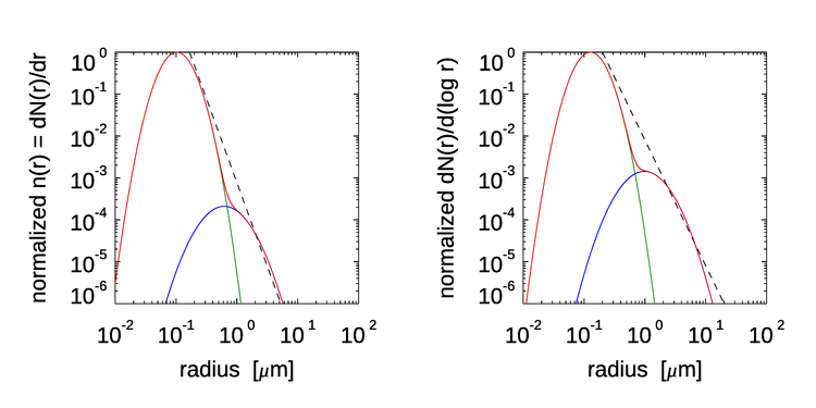
The parameters , and are adjusted to give the relative amounts of continental and marine aerosols, and the parameters also depend on the relative humidity. Figure illustrates these aerosol distributions for a typical open-ocean mix of aerosol types and for a relative humidity of 50%. The left panel plots the number PSD and the right panel plots the same information as . In the left panel, the dashed line shows the slope of a Junge distribution (Eq. 6). In the right panel, the Junge distribution is represented by a slope of on the abscissa sale (Eq. 5). The aerosol model of Eq. (9) uses particle radius rather than diameter because these particle size distributions are used as input to Mie calculations of aerosol optical properties.
The log-normal distribution finds many applications beyond particle size distributions. Campbell (1995) shows examples of log-normal distributions of chlorophyll concentrations, normalized water-leaving radiances, the diffuse attenuation coefficient , normalized photosynthetic yields, and several other biological variables. In fields other than oceanography, the log-normal distribution has been found to describe phenomena as diverse as the distribution of income (excluding billioniares), daily rainfall amounts, the populations of cities, and much more. Qualitative understanding of these observations can be obtained as follows. If a random variable is the sum of other random variables, then the distribution of the sum will be normal, regardless of the distribution of the individual variables. This is known as the Central Limit Theorem. (See the page on Error Estimation in Monte Carlo calculations for numerical examples.) If the total results from a product of random processes, then the product will obey a log-normal distribution. This is because the logarithm of a product is the sum of the logarithms, and the sum of the individual logarithms is then normally distributed. Thus, for example, if the total chlorophyll concentration is the result of a repeated daily fractional increase (daily growth rate) (e.g., the total Chl is the value at day 1 times 1.1 to get the value at day 2, time 1.1 again to get the value at day 3, ...), the the total chlorophyll concentration will be log-normally distributed.
Comments on Units
Suppose you have some data that you wish to model with a normal or Gaussian distribution. might the the number, area, or volume of particles, and is some measure of their size. The mean and standard deviation of the data are and , respectively, and is the total “amount” of for all sizes (e.g., the total number of particles or their total volume). Then the Gaussian model of the data would be
| (10) |
If has units, say , then and have the same units. The argument of the exponential is nondimensional, and
since a Gaussian distribution integrates to 1.
Now suppose you wish to model the same data using a log-normal distribution. The idea is that
| (11) |
where now and are the parameters of the distribution. However, this equation is not correct because you cannot take the logarithm of a dimensional quantity. (Nor can you compute or or any other such function unless is a nondimensional number.) However, you can compute if has units of 1 over the units of , so that is a nondimensional number. Thus, before using a log-normal distribution, you must non-dimensionalize the size . If is in , then this can be done by dividing all values of by , i.e. setting . However, you could just as well normalize the values by dividing by . Note that converting the data values from, say, micrometers to millimeters, or even to inches, also amounts to multiplying all values by a scale factor . If , then and , and the exponential of the log-normal distribution does not change. The log-normal distribution this then properly written as
| (12) |
where now and . Of course, if is measured in micrometers and , then nothing changes numerically in Eq. (11) vs. (12), but it should be kept in mind when using equations like (8) or (9) that the size measure or must be non-dimensional. This subtlety seems never to be mentioned in the particle sizing literature, although the mathematicians have commented on this; see Matta et al. (2011) and Finney (1977).
Single-parameter measures of particle size
A PSD contains the full information about the sizes of particles in a sample. However, a PSD is a function of size, and there is a human tendency to want to have a single number to describe the particle sizes. Using a single number to describe a distribution may sometimes be useful, but it often can be misleading or downright dangerous. As shown in the introduction, it is not even possible to define a unique “size” for more than one sphere, let along a distribution of non-spherical particles. A power-law distribution diverges as the size goes to 0, so such a distribution can be integrated only over a finite size range to . Numbers like the mean or median particle size can be computed for a distribution, but the “mean” size will be different when based on a number distribution versus a volume distribution, for example.
Perhaps the most commonly used single-number size parameter is the Sauter mean diameter (SMD), which is defined by
Recalling Eqs. 3 and 4, the SMD can be written as , where and are the total volume and area of the particles in the distribution. For a single spherical particle of volume and area , the SMD reduces to the diameter of the sphere. Thus in words, the SMD is the diameter of a sphere that has the same total volume to total area ratio as the particles in the distribution.
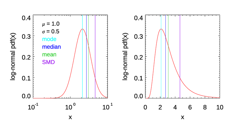
Figure 7 shows the differences in the mode, median, mean, and Sauter mean diameter for a log-normal probability distribution function,
with parameters and . This illustrates that these measures of particle “size” are in general all different. The Sauter mean diameter is larger than the others and is determined most strongly by the largest particles of a distribution. If you are interested in total volume or mass, then the SMD is a useful quantity. This is why the SMD is used in sediment transport studies. On the other hand, if you are interested in the smallest particles, then the mode or median is probably a better statistic to use. Other single-number measures of a distribution have been developed for specific problems. Clearly, which single measure of a size distribution might be most useful depends on the problem at hand.
 See comments posted for this page and leave your own.