Autocovariance Functions: Theory

The preceding pages have described the statistical properties of random sea surfaces using variance spectra. This page begins the exploration of an alternate path to the specification of surface roughness properties. Clearly, wind-dependent variance spectra are applicable only to surface waves that are generated by wind. Consider, however, the surface of a flowing river. The river’s surface can have ripples or waves generated by turbulence resulting from unstable shear flow induced by flow over a shallow bottom, or by eddies created as the water flows around rocks in the river. These water surfaces do not depend on the wind speed and can have different statistical properties, hence different optical properties, than wind-roughened water surfaces. Such surfaces can be described by their autocovariance functions.

Autocovariance functions can be converted to elevation variance spectra via the Wiener-Khinchin theorem. This page shows how that is done. Once a given autocovariance function has been converted to its equivalent elevation variance spectrum, the algorithms of the previous chapters are immediately applicable, even though the variance spectrum is not wind-dependent. Indeed, this conversion enables the Fourier transform methods of the previous chapters to be used to generate random realizations of any surface, not just water surfaces.

As is often the case, there is a large gap between textbook theory—usually developed for continuous variables or an infinite sample size of discrete values—and its implementation in a computer program for a finite sample size of discrete variables. In particular, careful attention must be paid to sampling of an autocovariance function in order to obtain the corresponding variance spectrum, or vice versa. I find it disappointing and frustrating (but not surprising) that numerical matters such as the effects of finite sample size, maximum lag size, and exactly how to sample spectra or autocovariances (in particular, the material on page Autocovariance Functions: Sampling) never seems to be mentioned in textbooks on digital signal processing or related subjects. It is left to the innocent student to spend a few weeks of unfunded time figuring out why various numerical results are not internally consistent or do not perfectly match the textbook theory.

This page begins with a discussion of autocovariances, and then the Wiener-Khinchin theorem is stated. The theorem is numerically illustrated on the next page first using the wind-dependent Pierson-Moskowitz elevation variance spectrum, for which certain values can be analytically calculated and used to check the numerical results. The modeling of water surfaces generated by shear-induced turbulence is then illustrated, again using analytical functions that allow for a rigorous check on the numerical results.

Autocovariance

The autocovariance $C_{zz}\left(\ell \right)$ of $z\left(r\right)$ is defined as

where $\mathcal{ℰ}$ denotes statistical expectation and $\ell$ is the spatial lag. This definition in terms of the expectation holds for both continuous and discrete variables. For the present discussion with $z\left(r\right)$ being sea surface elevation, $C_{zz}\left(\ell \right)$ shows how strongly the sea surface elevation at one location is correlated to the elevation at a distance $\ell$ away. $C_{zz}\left(\ell \right)$ has units of $m^2$, and $C_{zz}\left(\ell =0\right)$ is the variance of the surface elevation. The autocovariance is an even function of the lag: $C_{zz}\left(-\ell \right)=C_{zz}\left(\ell \right)$.

Consider an infinite sample of discrete zero-mean surface elevations spaced a distance $\Delta x$ apart. The autocovariance is then computed by (e.g., Eq. 2.6.3 of Proakis and Manolakis (1996) with a minor change in their notation)

Here $\ell$ is indexing the lag distance in units of the sample spacing $\Delta x$. For a finite sample of $N$ discrete values, the same authors define the sample autocovariance by (their Eq. 2.6.11)

As usual, there are competing definitions. For a finite sample of $N$ discrete values, perhaps with a non-zero mean $m$, the IDL autocorrelation function (A_CORRELATE) uses

where

is the sample mean. Matlab computes the autocovariance via

Note that the lag must be less than the length of the sample. (That is, the sample locations are at $x_r=r\Delta x,r=0,...,N-1$ and the allowed lag distances are ${\ell }_r=r\Delta x,r=0,...,N-2$.) Note also the factor of $1∕N$ in the IDL definition (3), which does not appear in Eq. (2), and which is a factor of $1∕\left(N-1\right)$ in the Matlab version.

Nor is there even any consensus on the terms “autocovariance” and “autocorrelation.” Some authors (and this page) define the nondimensional autocorrelation ${\rho }_{zz}\left(\ell \right)$ as the autocovariance normalized by the variance, i.e.

However, Proakis and Manolakis (1996) call the autocovariance as used here the autocorrelation, and they call the autocorrelation of Eq. (4) the “normalized autocorrelation.” These sorts differences in the definitions and computations of autocovariances can can cause much grief when comparing the numerical outputs of different computer codes, or numerical outputs with textbook examples.

The Wiener-Khinchin Theorem

Now that the autocovariance has been defined, the Wiener-Khinchin theorem can be stated: The Fourier transform of the autocovariance equals the variance spectral density function. Symbolically,

Indeed, some texts define the spectral density as the Fourier transform of the autocovariance. The inverse is of course

Here ${\mathcal{𝒮}}_{2s}$ is a two-sided spectral density function as discussed on several previous pages (e.g., Surfaces to Spectra: 1D).

It is important to note (as emphasized by the $\nu$ subscript on the Fourier transform operator $\mathcal{ℱ}$) that the theorem is written with the $\nu$ version of the Fourier transform (Eq. 1 of the Fourier Transforms page), and the density function is written in terms of the spatial frequency $\nu$, which has units of 1/meters. (In the time domain, the conjugate variables are time $t$ in seconds and frequency $f$ in 1/seconds = cycles/second = Hz.) The spectral density function for the angular spatial frequency $k=2\pi \nu$ (or angular temporal frequency $\omega =2\pi f$ in radians per second in the time domain) can be obtained by noting that corresponding intervals of the spectral densities contain the same amount of variance:

which gives

Note that $\ell$ varies from $-\infty$ to $+\infty$ and, likewise, $\nu$ or $k$ ranges over all negative and positive values. The variance spectrum obtained from the Fourier transform of an autocovariance function is therefore a two-sided spectrum.

Comment: In light of Eq. (7), the theorem stated in terms of angular spatial frequency $k$ appears to be

with the inverse

I say “appears to be” because I’ve never actually seen the theorem written this way because the textbooks all seem to stick with $x$ and $\nu$ (or $t$ and $f$ in the time domain). As Press et al. (1992) say in Numerical Recipes (p. 491), “There are fewer factors of $2\pi$ to remember if you use the ($\nu$ or) $f$ convention, especially when we get to discretely sampled data....” In any case, Eqs. (8) and (9) are consistent with the $k$ spectrum of Eq. (17) discussed below.

The theorem is usually proved in textbooks for continuous variables $x$ and $\nu$. However, in numerical application to a finite number of discrete samples, discrete variables $x_r$ and ${\nu }_u$ or $k_u$ are used, and proper attention must be paid to pesky factors of $N$, $2\pi$, and bandwidth, and to the array ordering required by a particular FFT routine.

The continuous-variable Fourier transform in Eq. (5) gives a spectral density ${\mathcal{𝒮}}_{2s}\left(\nu \right)$ with units of $m^2∕\left(1∕m\right)$. However, if the theorem is written for a DFT of discrete data $C_{zz}\left({\ell }_r\right)=C_{zz}\left(r\right)$,

then the resulting discrete spectrum ${\mathcal{𝒮}}_{2s}\left({\nu }_u\right)={\mathcal{𝒮}}_{2s}\left(u\right)$ has units of $m^2$. Just as was discussed on the Fourier Transforms page, this discrete spectrum must be divided by the bandwidth $\Delta \nu$ in order to obtain the density at $\nu ={\nu }_u$. That is,

Example

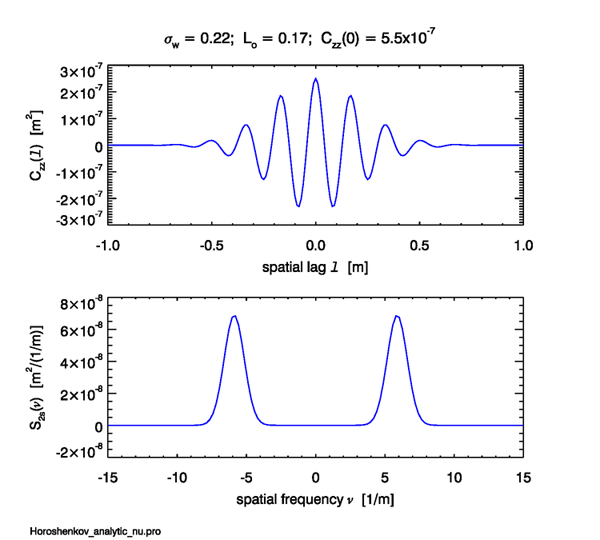
Horoshenkov et al. (2013) (their Eq. 4) give an analytic formula for the autocorrelation function of surface waves generated by bottom-induced turbulence in shallow flowing water. In the notation of this page, this function is

In their words, “${\sigma }_w$ relates to the spatial radius of correlation (correlation length)” and “$L_o$ relates to the characteristic period in the surface wave pattern.” The average values for the physical conditions of the Horoshenkov et al. study are ${\sigma }_w=0.22m$ and $L_o=0.17m$. [Note: Eq. (12) is Horoshenkov’s $W\left(\rho \right)$ as shown in their abstract and in their conclusions, where it has a factor of 1/2 in the exponential. Their Eq (4) does not have the 1/2. This is probably a typo since Gaussians usually have the form $exp\left[-x^2∕\left(2{\sigma }^2\right)\right]$.]

This autocorrelation function provides a nice example of how to use the Wiener-Khinchin theorem to obtain the corresponding variance spectrum. Equation (12), when converted to an autocovariance via a factor of the variance, $⟨z^2⟩=C_{zz}\left(0\right)$, has the form

where $a=1∕\left(\sqrt{2}{\sigma }_w\right)$ and $q_o=2\pi ∕L_o$. This function has an easily computed analytical Fourier transform.

The continuous-variable Fourier transform of this $C_{zz}\left(\ell \right)$ is given by Eq. (1) of the Fourier Transforms page:

Here $\ell$ and $\nu$ are continuous variables; ${\mathcal{𝒮}}_{2s}\left(\nu \right)$ has units of $m^3$, which is interpreted as $m^2∕\left(1∕m\right)$ as explained before. Note that this variance spectral density is two-sided, i.e., $\infty <\nu <\infty$. Expanding the complex exponential via $e^{-i𝜃}=cos𝜃-isin𝜃$ gives

The imaginary term is zero because the integrand is an odd function of $\ell$. Using the identity

gives

The integral

gives the Fourier transform of the $C_{zz}\left(\ell \right)$ of Eq. (13):

This variance spectrum has maxima at $\nu =\pm 1∕L_o$, where the value is very close to $\sqrt{\frac{\pi }{2}}{\sigma }_w{C}_{zz}\left(0\right)$. Figure 1 plots this $C_{zz}\left(\ell \right)$ (Eq. 13) and ${\mathcal{𝒮}}_{2s}\left(\nu \right)$ (Eq. 15) for typical values of ${\sigma }_w=0.22m$, $L_o=0.17m$, and $C_{zz}\left(0\right)=2.5\times 10^{-7}{m}^2$. Note that the sub peaks of the autocovariance lie at integer multiples of $\pm L_o$, and that the peaks of the spectrum are at $\pm 1∕L_o$.

By definition, the integral over all frequencies of an elevation variance spectral density gives the total elevation variance $⟨z^2⟩$:

This can be computed analytically for the spectrum of Eq. (15). The ${\mathcal{𝒮}}_{2s}\left(\nu \right)$ spectrum of Eq. (15) is the sum of two identical Gaussians centered at different $\nu$ values. Consider the one centered at $\nu =1∕L_o$, which involves the exponential with the $\nu -1∕L_o$ term. The total variance is then twice the integral of this Gaussian:

Letting $x=\nu -1∕L_o$ gives

where $c^2=\frac{1}{2}{\left(2\pi {\sigma }_w\right)}^2$. The integral

then gives the final result:

Thus starting with a variance of $C_{zz}\left(0\right)$ in the autocovariance of Eq. (13), obtaining the variance spectral density from the Fourier $\nu$-transform of the autocovarience, and then integrating the variance spectral density over $\nu$ thus gives back the variance as originally specified in the autocovariance function.

However, if the above process is naively carried through starting (as in Eq. 14) with the $k$-transform of Eq. (3) on the Fourier Transforms page, the end result (as in Eq. 16) is $2\pi C_{zz}\left(0\right)$. This extra factor of $2\pi$ is rectified by the $1∕2\pi$ factor seen in Eq. (7). Thus the $k$ version of the Horeshenkov spectral density is

Integration of this ${\mathcal{𝒮}}_{2s}\left(k\right)$ over all $k$ then results in $⟨z^2⟩=C_{zz}\left(0\right)$, as required. The inverse $k$ transform of the spectral density (17) gives $C_{zz}\left(\ell \right)∕\left(2\pi \right)$, as expected from Eq. (9).