Page updated:
March 13, 2021
Author: Collin Roesler
View PDF
Non-Algal Particles (NAP)
As noted in the introduction to this chapter, the term non-algal particles (NAPs) refers to particulate matter that does not have extractable (via solvents such as acetone or methanol) pigments. This includes all living and detrital organic matter such as the non-pigmented portion of phytoplankton cells, detritus, heterotrophic bacteria, and viruses. Many authors also include inorganic mineral particles of both biogenic (e.g., calcite liths and shells) and terrestrial origin (e.g., clay, silt, and sand).
Detritus
Detritus is a catch-all term for non-living particulate organic matter, including dead bacterial, phytoplankton and zooplankton cells, fragments of cells left from zooplankton grazing, fecal pellets, shells, and marine snow aggregates. Detritus both absorbs and scatters and can constitute an important fraction of the total IOPs of a water body.
Absorption by detritus
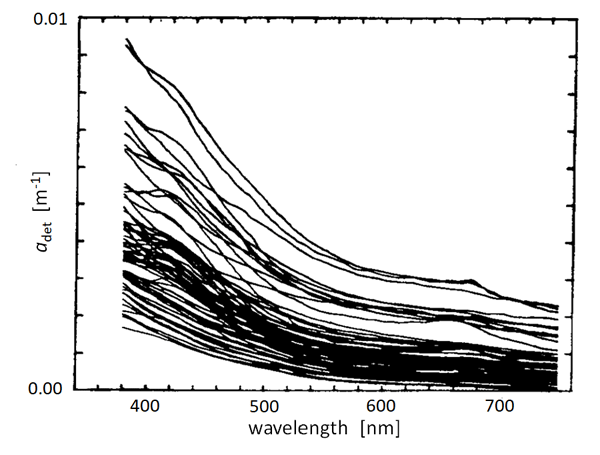
There have been many measurements of the absorption spectra of detritus and NAPs. Figure 1 shows an example. These measurements include both biogenic detritus and whatever mineral particles (if any) were in the water. Although magnitudes vary greatly depending on the concentration of NAPs in the water, the curves show a generally exponential decay with increasing wavelength. It is thus common (Kirk (1980), Roesler et al. (1989), Bricaud et al. (1998)) to model absorption by detritus or NAPs via
| (1) |
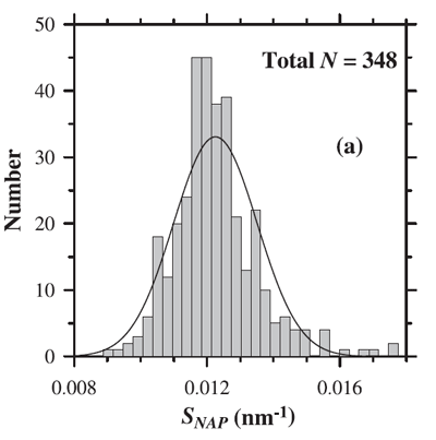
where is a reference wavelength and the spectral slope parameter. The mean value of used to model NAP absorption is (e.g., Roesler et al. (1989), Bricaud et al. (1998)). However, as always with data-derived parameters, there is variability in . Figure 2 shows the distribution of values observed by Babin et al. (2003b). Their data show a mean of with a standard deviation of 0.0013.
The absorption model of Eq. (1) has the same functional form as that for absorption by CDOM, although the average spectral slope parameter differs somewhat from the average parameter for CDOM, ; see Commonly Used Models for IOPs and Biogeochemistry.
Scattering by detritus
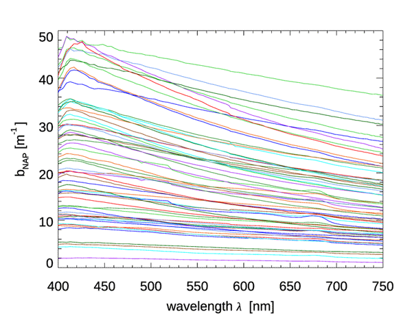
Although CDOM and NAPs have similar absorption spectra, they differ greatly in their scattering properties: CDOM has negligible scattering, but NAPs can be strongly scattering. There is much less data on NAP scattering than for absorption, but Fig. 3 shows data from Great Lake (Taihu), China. The spectra in this dataset show a rather featureless dependence on wavelength, which is well fit () by a power law:
| (2) |
The authors show that the IOPs of this lake are dominated by NAP, with phytoplankton usually contributing less that 10% of the total scattering. (The same dataset had NAP absorption spectra that were well fit by Eq. (1), but with a spectral slope parameter of , which is about one-half of typical ocean values.)
Minerals
Mineral particles can enter the ocean from river discharge, erosion of coastal cliffs, sediment resuspension, and deposition of atmosphere dust, which is often carried long distances by winds. The optical properties of such particles are just as varied, and often just as important, as the properties of biological particles. In spite of their importance, relatively few studies have investigated the absorption and scattering properties of minerals per se. These include Ahn (1999), Stramski et al. (2004), Babin and Stramski (2004), and Stramski et al. (2007).
Absorption by minerals
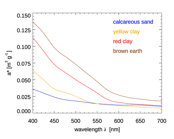
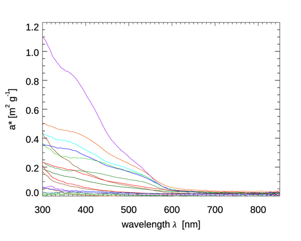
Figure 4 shows mass-specific absorption coefficients (units of ) for four types of minerals. Figure 5 shows the same for several types of mineral dust suspended in sea water; some of the curves are the same mineral type but with different particle size distributions. The imaginary indices of refraction for these particles varied by an order of magnitude, from about 0.003 to 0.03, depending on wavelength and mineral type. See Stramski et al. (2007) for a full discussion. These (and other) data sets are in qualitative agreement: absorption by minerals can range from highly absorbing in the blue with a roughly exponential decrease with increasing wavelength, to almost non-absorbing and spectrally flat. Thus, to first order, absorption by minerals can be modeled by either an exponential,
or a power law,
where is a reference wavelength. The parameters and can be adjusted as needed to fit a particular mineral type.
Scattering by minerals
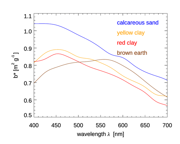
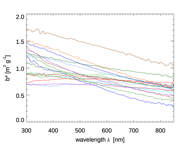
Figures 6 and 7 show the mass-specific scattering coefficients for the same two data sets of Figs. 4 and 5. As for absorption, the scattering coefficients show a decrease from blue to red, although with a couple of notable exceptions for the brown earth and Kosan samples, which have their maximum values at green wavelengths. Many of these scattering coefficients could be modeled with an exponential or power law function. However, in all cases, use of a measured spectrum for radiative transfer calculations is preferable.
Stramski et al. (2001) used complex indices of refraction for detritus and mineral particles, a power law particle size distribution with a slope parameter of -4 (a Junge distribution), and Mie theory to compute absorption, scattering, and backscattering cross sections for detritus and minerals. Their results are shown in Table 1. It is interesting to note how closely the wavelength exponents for the scattering cross sections agree with the best-fit values for the NAP-dominated waters of Fig. 3 as seen in Eq. (2).
| Component | Absorption | Scattering | Backscattering |
| Detritus | |||
| Minerals | |||
 See comments posted for this page and leave your own.