Spectra to Surfaces: 1D

The previous page showed the major features of the Fourier analysis of a sea-surface elevation record. We started with a sample of a random sea surface and ended with the corresponding discrete variance spectrum (or estimate of the variance spectral density after division by the frequency interval). This page shows how to go in the reverse direction: start with a variance spectrum and generate a random realization of the corresponding sea surface. We first outline the theory, and then show a specific example.

Theory for 1-D Surfaces

To create a one-dimensional (1-D) slice through a sea surface, the essence of the process is as follows:

1.

Choose the domain size. To create a sea surface over a spatial domain at a given time, we pick the length $L$ of the region $\left[0,L\right]$. To generate a time series at a given point, we pick the length of the time series.

2.

Choose the number of points for the DFT. This number $N$ is the number of frequencies at which we will sample the variance spectrum, and equals the number of samples of the sea surface that will be generated. In normal usage, pick $N$ to be a power of 2 so that an inverse FFT routine can be used to evaluate the inverse DFT.

3.

Choose the frequency variable. To generate a sea surface over a spatial domain at a given time, we can use either wavenumber $\nu$ or angular spatial frequency $k$. To generate a time series at a given point, we can use either $f$ or $\omega$.

4.

Choose a variance spectrum The variance spectrum must be expressed in terms of the chosen frequency variable.

5.

Choose the wind speed. Pick a wind speed, and perhaps other physical parameters such as the age of the waves to be generated if required by the chosen variance spectrum.

6.

Create random Hermitian amplitudes. This is the tricky part. We must create an array of randomized discrete Hermitian Fourier amplitudes $ẑ\left(u\right)$, starting with the chosen continuous variance spectrum.

7.

Take the inverse DFT of the random amplitudes. The inverse DFT converts the Fourier amplitudes to the physical wave heights.

8.

Extract the sea surface heights. The inverse DFT of the complex amplitudes returns a complex array. The real part of this array is the random realization of the sea surface heights, and the imaginary part is zero.

9.

Check your results. This is extremely important during code development. For example, take the DFT of the generated surface heights to see if you get back to the Fourier amplitudes and variance spectrum you started with.

We now proceed through these steps and discuss them in detail for a specific example.

Steps 1 and 2: Let us generate a sea surface over the region from $x=0$ to $x=L=100m$. The longest wavelength that can be resolved is then 100 m. We use $N=1024$, which gives a spatial grid resolution of $\Delta x=L∕N=0.0977m$. This means that the shortest wavelength that can be resolved, the two-point wave or Nyquist wavelength, is $2\Delta x=0.1954m$.

Step 3: We used wavenumber $\nu$ in the previous pages because of its easy interpretation. Now let’s use angular spatial frequency $k$, which is more commonly used. The fundamental frequency is then $k_f=2\pi ∕L=0.0628rad{m}^{-1}$. The highest frequency sampled, the Nyquist frequency, is $k_{Ny}=\left(N∕2\right)k_f=32.15rad{m}^{-1}$. Note that $\left(2\pi \right)∕k_{Ny}=0.1954m$ which, as noted above, is the wavelength of the two-point wave.

Step 4: For this example, we use the Pierson-Moskowitz variance spectrum in terms of angular spatial frequency $k$. This is given by Eq. (1) of the Wave Variance Spectra: Examples page. Note that this is a one-sided spectrum, which is defined for positive $k$ values.

Step 5: The wind speed at 10 m elevation is $U_{10}=5m{s}^{-1}$. The wind speed is the only input to the Pierson-Moskowitz spectrum.

Step 6: We now discuss in detail how to generate a set of random discrete Fourier amplitudes that are physically consistent with the chosen variance spectrum. These amplitudes must be defined for both positive and negative frequencies, and the amplitudes must be Hermitian. We first define

Here ${\mathcal{𝒮}}_{1s}\left(k=k_u\right)$ denotes the continuous spectral density ${\mathcal{𝒮}}_{1s}\left(k\right)$ evaluated at $k=k_u$. $\Delta k=k_f$ is the spatial frequency sampling interval. ${ẑ}_o\left(k_u\right)$ must be defined for both positive and negative discrete frequencies in order to create the Hermitian amplitudes for use in the inverse DFT. As was mentioned on the previous page, we must convert the one-sided continuous spectrum ${\mathcal{𝒮}}_{1s}\left(k\right)$ into a two-sided discrete variance function by

1.

dividing its magnitude by 2, assuming that ${\mathcal{𝒮}}_{2s}\left(-k\right)={\mathcal{𝒮}}_{2s}\left(k\right)$;

2.

multiplying the continuous spectral density by the fundamental frequency interval $\Delta k$, which gives the variance contained in a finite frequency interval at each frequency $k_u$.

To emphasize the discrete vs continuous functions, and for brevity of notation, let us write the frequency index $u$ for the frequency $k_u$. Then Eq. (1) becomes

where ${\mathcal{𝒮}}_{2s}\left(u\right)$ denotes the two-sided discrete variance spectrum at frequency $k_u$. ${ẑ}_o\left(u\right)$ can now be evaluated for both positive and negative $k_u$. The 0 and Nyquist frequencies are always special cases: set ${\mathcal{𝒮}}_{2s}\left(0\right)=0$ and ${\mathcal{𝒮}}_{2s}\left(k_{Ny}\right)={\mathcal{𝒮}}_{1s}\left(k_{Ny}\right)$. $\rho \left(k_u\right)\equiv \rho \left(u\right)$ and $\sigma \left(k_u\right)\equiv \sigma \left(u\right)$ are independent random numbers drawn from a normal distribution with zero mean and unit variance, denoted $\rho ,\sigma \sim \mathcal{𝒩}\left(0,1\right)$. A different pair is drawn for each $u$ value.

${ẑ}_o\left(u\right)$ is a random variable. Let $⟨...⟩$ denote the expectation of the enclosed variable. The expected value of $|{ẑ}_o\left(u\right){|}^2$, $⟨{ẑ}_o\left(u\right){ẑ}_o^{\ast }\left(u\right)⟩$, gives back whatever variance function is used for ${\mathcal{𝒮}}_{2s}\left(u\right)$:

because $⟨{\rho }^2⟩=⟨{\sigma }^2⟩=1$ for $\mathcal{𝒩}\left(0,1\right)$ random variables. Thus ${ẑ}_o\left(u\right)$ is consistent with the chosen variance spectrum. However, ${ẑ}_o\left(u\right)$ is not Hermitian, so the inverse DFT would not give a real sea surface.

Next define $ẑ\left(u\right)$ as

This function is clearly Hermitian, so the inverse DFT applied to $ẑ\left(u\right)$ will give a real-valued $z\left(x_r\right)\equiv z\left(r\right)$. Moreover, this $ẑ\left(u\right)$ is consistent with the variance spectrum:

Here we have noted that $⟨\rho \left(u\right)\rho \left(-u\right)⟩=0$, etc., because the random variables are uncorrelated for different $u$ values.

Equations (1) and (3) are the key to generating random sea surfaces from variance spectra. $ẑ\left(u\right)$ defined by these equations contains random noise, which leads to a sea surface with random amplitudes and phases for the component waves of different frequencies. Any one of these surfaces has a variance spectrum that looks like the chosen spectrum plus random noise. However, on average over many realizations, the the noise in these spectra will average out, leaving the variance spectrum. Figure 1 below illustrates these important ideas, but first we must complete the surface generation.

Step 7: Compute the inverse DFT of the $ẑ\left(u\right)$ of Eq. (3). The result is a complex function $Z\left(x\right)$:

A crucial warning to this step is that the $u=0,...,N-1$ elements of the $ẑ\left(u\right)$ array must be in the FFT frequency order given by Eq. (13) of the Fourier Transforms page when using an FFT routine to evaluate the DFT. $Z\left(r\right)$ is returned with $x_r$ values in the order from $x_0=0$ to $x_{N-1}=\left(N-1\right)\Delta x$.

Step 8: Extract the surface. The inverse DFT returns a complex array $Z\left(x_r\right)$ whose real part is the surface elevations $z\left(x_r\right)$ and whose imaginary part is 0. The surface elevations are extracted as the real part of $Z\left(x_r\right)$:

Step 9: Check the results! There are many places along the way to lose a $\sqrt{2}$ or to mess up array indexing. At the minimum, it is worthwhile to check that the mean of the generated surface is zero, and that the imaginary part of $Z\left(x_r\right)=0$ (to within a small amount of numerical roundoff error).

When developing computer code, or when first learning this material, it is also a good idea to take the forward DFT of $Z\left(x_r\right)$ to make sure that the input Fourier amplitudes $ẑ\left(u\right)$ are recovered, and that the variance spectrum corresponding to $z\left(x_r\right)$ is consistent with the one chosen in Step 4. Indeed, it was the failure of this check in surfaces I was generating using equations from the literature that led me to develop the Mobley (2016) tutorial and these web pages.

Equations (1) and (3) are, with minor changes in notation, Eqs. (42) and (43), respectively, of Tessendorf (2004). However, Tessendorf’s version of Eq. (1) appears to use a one-sided variance spectrum (his example used the one-sided Phillips spectrum of his Eq. (40)) without the division by 2 seen in Eq. (1), which is needed to convert the one-sided spectrum to a two-sided spectrum. Nor does he show the $\Delta k$ factor needed to convert a continuous spectral density to a discrete function. His version of Eq. (3) does not contain the overall factor of $1∕\sqrt{2}$ seen above. These missing factors mean that in a round-trip calculation

you do not get back to the original variance spectrum. In other words, the Tessendorf equations do not conserve wave variance (i.e., wave energy). Even if he included the $\Delta k$ factor in his actual computations, the missing factors of $1∕\sqrt{2}$ in his versions of our Eqs. (1) and (3) give an overall factor one-half on the amplitudes, which corresponds to a factor of four error in the variance. That is, waves generated using the Tessendorf equations have amplitudes that are too large.

Tessendorf (2004) discusses much more than just Fourier transform techniques, and his notes have been very influential in the computer graphics industry. In 2008 he deservedly received an Academy Award for Technical Achievement for showing the movie industry how to generate and render sea surfaces, as well as for his many other pioneering accomplishments in efficiently computing and rendering fluid motions into visually appealing images. (The first movie to use his techniques was Waterworld, followed by dozens of others including Titanic.) When I checked with him about the missing numerical factors, he readily acknowledged that Eqs. (1) and (3) are the correct ones, but pointed out that “Hollywood doesn’t care about conservation of energy.” I suppose that should be no surprise, since movies seem to have no problem with rockets going faster than the speed of light, sound propagating through the vacuum of outer space, or time travel that violates causality. Tessendorf’s equations are widely cited (especially in the computer graphics literature), always without comment about the missing scale factors. Even if Tessendorf had included the needed numerical factors in his equations, graphics artists would distort the resulting images to make them look “better,” e.g., to make the ocean waves look bigger than nature would allow. That may be acceptable in a fantasy world, but such laxness is not permissible if we wish to use numerically generated waves to compute sea surface optical properties.

Example: A Roundtrip Calculation

Figure 1 shows an example of 1-D surface waves generated using the Pierson-Moskowitz spectrum for a wind speed of 5 m/s, and the recovery of the variance spectrum from the generated surface. The blue curve in the upper-left panel shows the Pierson-Moskowitz spectrum as defined by Eq. (1) on page Wave Variance Spectra: Examples. The red dots show the frequencies at which the continuous spectrum is sampled. Those dots blur together at the higher frequencies because of the log scale, but the $k_u$ points are equally spaced at intervals of the fundamental frequency $\Delta k=k_f=2\pi ∕L=0.0628rad∕m$. The last sampled frequency is $k_{Ny}=32.17rad∕m$. The bottom panel shows the sea surface elevations $z\left(x_r\right)$ generated for a particular sequence of random numbers $\rho \left(u\right),\sigma \left(u\right)$.

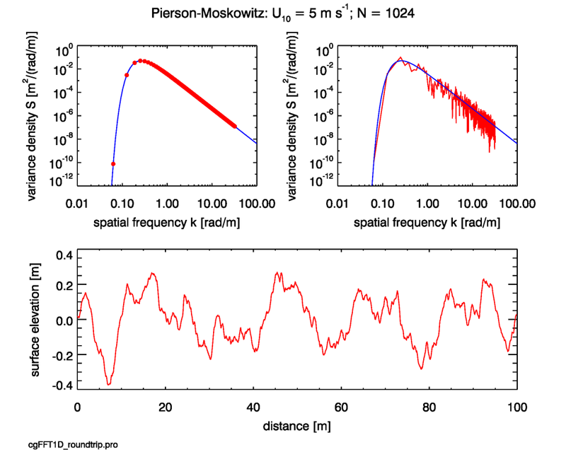
The red line in the upper-right panel shows the function

$\mathcal{𝒫}\left(u\right)$ is the discrete variance function for this particular $z\left(x_r\right)$ surface. Schuster (1898) called $\mathcal{𝒫}\left(u\right)$ a periodogram. The periodogram $\mathcal{𝒫}\left(u\right)$ contains random noise because $z\left(x_r\right)$ is a random realization of the sea surface, which was generated by applying random noise to the the variance spectrum. This particular $z\left(x_r\right)$ is analogous to a particular measurement of the sea surface. Had we drawn a difference sequence of random numbers for use in Eq. (2), we would have generated a different sea surface, and a different $\mathcal{𝒫}\left(u\right)$. However, we can expect that if we average together many different $\mathcal{𝒫}\left(u\right)$, corresponding to many different sets of $z\left(x_r\right)$, the noise would average out and we would be left with a curve close to the variance spectrum we started with, which is shown in blue. Numerical experimentation shows that averaging 100 $\mathcal{𝒫}\left(u\right)$ generated from 100 independent sea surface realizations gives an average $\mathcal{𝒫}\left(u\right)$ that is almost indistinguishable from the blue curve at the scale of this plot. Thus $\mathcal{𝒫}\left(u\right)\equiv \mathcal{𝒫}\left(k_u\right)$ is an approximation of the variance density spectrum $\mathcal{𝒮}\left(k\right)$, denoted $\mathcal{𝒫}\left(k_u\right)\doteq \mathcal{𝒮}\left(k\right)$. This averaging processes leads to the topic of spectrum estimation, which considers such problems as how many sets of measurements of $z\left(x_r\right)$ are needed to estimate the variance spectrum to within certain error bounds. Fortunately, we need not pursue that here. (The noise is the upper right panel is Gaussian distributed about the theoretical spectrum. However, the log axis makes it look asymmetric about the blue curve.)

At the minimum, you should always check to see that Parseval’s relation, Eq. (17) of the Fourier Transforms page, is satisfied. For the simulation of Fig. 1, we have

There are sometimes other checks that can be made. For example, the Pierson-Moskowitz spectrum is simple enough that it can be analytically integrated over all frequencies. This gives

where we have recalled that the variance spectral density is related to the variance of the sea surface. The variance of the generated zero-mean sea surface can be computed from

and compared with the analytical expectation. For the surface seen in Fig. 1, Eq. (6) gives $var\left\{z\right\}=0.0189m^2$ vs. the theoretical value of $⟨z^2⟩=0.0197m^2$ from Eq. (5). This agreement to within a small amount of random noise indicates that all is probably well with the calculations. Indeed, the average $var\left(z\right)\pm$ one standard deviation for 100 independent simulations is $0.020\pm 0.007$, which agrees well with the theoretical value.

The significant wave height $H_{1∕3}$ is by definition the height (trough-to-crest distance) of the highest one-third of the waves. To a good approximation, this is related to the expectation of the variance by

In the present example, this formula gives $H_{1∕3}=0.55m$. The average significant wave height for 100 simulations is $0.56\pm 0.09$ (average $\pm$ one standard deviation). If you spend enough time in a sea kayak to develop intuition about wave heights as a function of wind speed, a half-meter height for the largest waves is about right for a $5m{s}^{-1}$ or 10 knot wind speed.

To summarize this page: we have learned how to start with a wave variance spectral density function and generate random discrete Fourier amplitudes. The inverse DFT of those amplitudes gives a random realization of a sea surface that is physically consistent with the chosen variance spectrum. That is all that we can ask of the Fourier transform technique.