Measuring IOPs

The definitions of the absorption and scattering coefficients on the Inherent Optical Properties page were in terms of an infinitesimally thin slab of water. We now must reformulate those conceptual definitions so that they can be applied to actual measurements on finite thickness of water in a measuring instrument.

Measuring The Beam Attenuation Coefficient

Just as was done for the absorption and scattering coefficients (recall Eqs. 1 and 2 of the IOP page), we can define the beam attenuation coefficient $c$ as

$$c\left(\lambda \right)=\frac{dC\left(\lambda \right)}{dr}\left(m^{-1}\right),$$

(1)

where $dC\left(\lambda \right)=dA\left(\lambda \right)+dB\left(\lambda \right)$ is the attenuance, or fraction of power absorbed or scattered as light passes through the slab of infinitesimal thickness $dr$. However, any instrument must make its measurements on a slab of some finite thickness $R$, which is typically between 0.01 and 1 m.

Figure 1 shows a finitely thick slab of water with an incident power ${\Phi }_{\text{i}}$ and transmitted power ${\Phi }_{\text{t}}$, where the wavelength argument has been omitted for brevity. Within the slab the power has magnitude $\Phi$ after passing through a thickness $r$ of material. In going from thickness $r$ to $r+dr$, the power changes from $\Phi$ to $\Phi +d\Phi$, where $d\Phi <0$ because the transmitted power decreases as the thickness traversed increases.

---

---

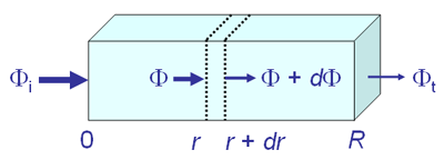
Recalling that the attenuance is the fractional change in power, we can rewrite Eq. (1) as

or

$$cdr=-\frac{d\Phi }{\Phi },$$

(2)

where the minus sign accounts for $d\Phi$ being negative, whereas all other quantities are positive. Assuming that the medium within the slab is uniform, so that $c$ is independent of $r$, we can integrate Eq. 2 from $r=0$ to $r=R$, which corresponds respectively to powers ${\Phi }_{\text{i}}$ and ${\Phi }_{\text{t}}$. This gives

which can be rewritten as

$$c=-\frac{1}{R}ln\left(\frac{{\Phi }_{\text{t}}}{{\Phi }_{\text{i}}}\right).$$

(3)

This equation gives the beam attenuation coefficient in terms of the measurable incident and transmitted powers and the finite thickness of the slab.

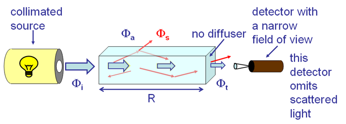
Equation (3) is the key to measuring the beam attenuation. However, there are additional subtleties in this measurement related to the instrument design, which is shown in more detail in Fig. 2. The development above implicitly assumed that the incident light was perfectly collimated (all light rays travel in exactly the same direction) and that the detector omits all scattered light. Neither requirement can be fully satisfied in a real instrument. Even a laser beam has some divergence, and any detector has a finite field of view (FOV) or acceptance angle. If the detector FOV is 1 deg, for example, then the detector will detect rays that have been scattered by 1 deg or less, as well as unscattered light. This undesired detection of scattered light will make the transmitted power too large, and thus $c$ too small. The magnitude of this error depends both on the detector FOV and on the volume scattering function of the water, which determines how much light is scattered through angles smaller than the FOV. Although these errors in beam attenuation measurements have been studied in many papers (see, most recently, Boss et al. (2009) and references therein), it is difficult to correct for the error in a particular measurement because the VSF is usually unknown, especially at very small scattering angles. Unfortunately, as Boss et al. show, the differences in $c$ values as measured by different instruments can be tens of percent. Indeed, Boss et al. end their paper with the comment, “We conclude that more work needs to be done with the oldest (in terms of availability of commercial in-situ instruments) and simplest (so we thought...) optical property, the beam attenuation.”

---

---

Measuring The Absorption Coefficient

If there were no scattering, then the instrument design used to measure beam attenuation would give the absorption coefficient $a$. However, at least some scattering is always present in sea water, which requires modification of the instrument design shown in Fig. 2. When measuring $a$, any light lost from the beam because of scattering will be attributed to a loss of light due to absorption. Thus it is desirable that the detector collect as much scattered light as possible. Because most scattering is through small angles, a common instrument design is to use as large a detector as possible at the end of the measurement chamber to collect forward scattered light. Such an instrument is shown schematically in Fig. 3.

---

---

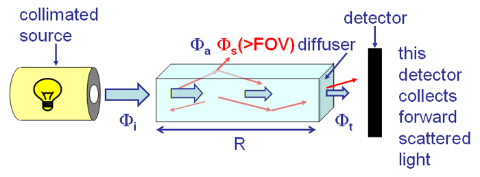
An instrument of this design typically collects light forward scattered through angles of a few tens of degrees (depending on the design of the particular instrument), which does account for most of the scattered light. However, some light is still lost “out the side of the instrument” by scattering though larger angles, as represented by ${\Phi }_{\text{s}}\left(>FOV\right)$ in the figure. To get an accurate absorption measurement, it is necessary to perform a scattering correction, i.e., to estimate ${\Phi }_{\text{s}}\left(>FOV\right)$ and to account for this loss when computing $a$. The equation for computation of $a$ then becomes

$$a=-\frac{1}{R}ln\left(\frac{{\Phi }_{\text{t}}+{\Phi }_{\text{s}}\left(>FOV\right)}{{\Phi }_{\text{i}}}\right).$$

(4)

In this equation, ${\Phi }_{\text{t}}$ now includes the measured transmitted power due both to unscattered light and to light scattered through angles less than the detector FOV. The ${\Phi }_{\text{s}}\left(>FOV\right)$ term adds back the unmeasured loss of power due to scattering through angles larger than the FOV. Estimating the value of ${\Phi }_{\text{s}}\left(>FOV\right)$ is of course difficult because the amount of scattering at angles greater than the instrument field of view depends on the (usually unknown) volume scattering function. Techniques for doing this scattering correction are given in Zaneveld et al. (1994).

In spite of the fundamental difficulties associated with the instrument designs of Figs. 2 and 3, the problems are not insurmountable and instruments based on these designs are commercially available. For example, the pioneering and widely used ac-9 instrument (and its successor, the ac-s) uses these designs for measurement of $a$ and $c$. In the ac-9, the detector for measurement of $c$ has an acceptance angle of about 1 deg, and the detector for measurement of $a$ has an acceptance angle of about 40 deg.

Another way to account for scattering in absorption measurements is to place the entire measurement chamber inside an integrating sphere. An integrating sphere is a hollow sphere coated on the inside with a highly reflective white material (usually Spectralon, which has a reflectance greater than 99% at visible wavelengths and is a diffuse reflector). The inner surface of the sphere reflects incident light into all directions, which after many reflections makes the interior light field homogeneous and isotropic. Thus it is possible to measure the power at only one location within the sphere in order to compute the total power within the sphere. Integrating spheres are commonly used in laboratory spectrophotometers to collect the scattered light, and flow-through integrating-cavity absorption meters are now commercially available (e.g., PSICAM).

Comment. Equation 4 is often rewritten as

$$\begin{array}{llll}\hfill a=-& \frac{1}{R}ln\left(\frac{{\Phi }_{\text{t}}+{\Phi }_{\text{s}}\left(>FOV\right)}{{\Phi }_{\text{i}}}\right)& \hfill & \\ \hfill -& \frac{1}{R}ln\left(\frac{{\Phi }_{\text{i}}-{\Phi }_{\text{a}}}{{\Phi }_{\text{i}}}\right)=-\frac{1}{R}ln\left(1-A\right),& \hfill & \end{array}$$

after recalling the definition of the absorptance $A$. Using ${log}_{e}x={log}_{10}x∕{log}_{10}e$ to convert from natural to Naperian logarithms gives

where $D=-{log}_{10}\left(1-A\right)$ is called the optical density or absorbance. Spectrophotometers usually output their measurements as a value of $D$, from which $a$ can be computed according to the thickness $R$ of the sample volume.

Measuring The Scattering Coefficient

It is possible to measure the scattering coefficient $b$, for example by collecting all scattered power in an integrating cavity and then using

It is also possible to measure the volume scattering function and then obtain $b$ by integration of the VSF over all scattering angles. However, neither of these paths to $b$ is often taken.

The scattering coefficient $b$ is usually obtained from measurements of the beam attenuation $c$ and absorption coefficient $a$, and the definition of $c$:

$$b=c-a.$$

Note, however, that there is a philosophical problem here, even if the practical difficulties in measuring $a$ and $c$ can be overcome well enough to obtain usefully accurate values. The philosophical problem is that to obtain good values of $a$ and $c$, you need to know the VSF in order to correct for the finite-FOV errors in $c$ and to perform the scattering correction for the $a$ measurement. Because the VSF is seldom measured, you must make assumptions about the scattering in order to obtain values for $a$ and $c$, in order to obtain a value for the scattering $b$. Thus the value obtained for the scattering coefficient depends on the a priori assumptions made about scattering in the water being studied. This circular reasoning is tolerated in optical oceanography simply because of the difficulties of designing instruments to make accurate measurements of each IOP independent of assumptions about the other IOPs.

Measuring The Volume Scattering Function

As with the measurement of beam attenuation, measurement of the volume scattering function employs a narrow collimated beam and a narrow-field-of-view detector. Now, however, the detector views the incident beam at a given scattering angle. The basic geometry is shown in Fig. 4.

---

---

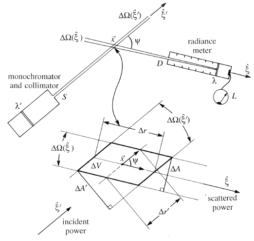
The intersection of the incident beam and the detector FOV define a volume of water $\Delta V$ in which the scattering from the incident direction ${\widehat{\xi }}^{\prime }$ into the scattered direction $\widehat{\xi }$ takes place. The scattering angle $\psi$ is defined as shown by the angle between ${\widehat{\xi }}^{\prime }$ and $\widehat{\xi }$ (recall Eq. (5) of the page on geometry). The incident power ${\Phi }_{\text{i}}$ traveling in direction $\widehat{\xi }$ into volume $\Delta V$ generates scattered power $\Delta {\Phi }_{\text{s}}\left(\psi \right)$ in the detector FOV of solid angle $\Delta \Omega$ centered on direction ${\widehat{\xi }}^{\prime }$ over a path length of $\Delta r$. The definitions of the VSF on The Volume Scattering Function page give us an operational formulas for the VSF in terms of measurable quantities:

$$\beta \left(\psi \right)=\frac{\Delta {\Phi }_{\text{s}}\left(\psi \right)}{{\Phi }_{\text{i}}\Delta r\Delta \Omega },$$

(5)

which as previously noted is equivalent to

$$\beta \left(\psi \right)=\frac{\Delta I_{\text{s}}\left(\psi \right)}{E_{\text{i}}\Delta V}.$$

(6)

As always, there are implicit assumptions and subtleties involved with these equations. It is assumed that the scattering volume $\Delta V$ is small enough that only single scattering takes place within the volume, but large enough to contain a representative sample of scattering particles. It is necessary to correct for attenuation of the incident and scattered beams along the entire path from the source to the scattering volume to the sensor, which presumes knowledge of the beam attenuation coefficient $c$. (Note again our problem: to measure the VSF we need to know $c$, but we need to know the VSF in order to make the FOV correction for the measurement of $c$.) In the pioneering General Angle Scattering Meter (GASM) developed by Petzold (1972), it was difficult to accurately determine the scattering volume $\Delta V$, which changes with scattering angle, because of the difficulty of maintaining mechanical alignment of the moving parts as they swept the detector through the full range of scattering angles. The calculations and engineering considerations needed to implement Eqs. 5 or 6 in GASM are given in Petzold’s classic report.

More recent instruments have used other designs to avoid various problems. For example, Lee and Lewis (2003) used a novel design based on a rotating periscope to scan through scattering angles from 0.6 to 177.3 deg. A more recent in situ instrument, the LISST-VSF can measure the VSF at 515 nm in the range of $\psi =0.094$ to 150 deg, along with the scattering coefficient and beam attenuation and selected components of the Mueller matrix for polarized light scattering. See Slade et al. (2013).

In sea water both absorption and scattering are always important. Depending on the water constituents and the wavelength, one process can dominate the other, but neither can be ignored. Thus one IOP cannot be measured independently of the others. Clearly, there is need for continued development of IOP instruments with novel designs that minimize the measurement problems mentioned above.