Page updated:
April 10, 2021
Author: Curtis Mobley
View PDF
Light from the Sun
This section briefly surveys how light is produced by the Sun, and characterizes the sunlight reaching the Earth.
The Proton-Proton Cycle
Since most of the light falling upon the earth originates in the Sun, it is worthwhile to start with a brief look at how this light is generated deep within the Sun in a process known as the proton-proton cycle. The core of the Sun is primarily a mixture of completely ionized hydrogen and helium. At the center the temperature is approximately , and the density is about 150 times that of water. Under these extreme conditions the hydrogen nuclei, or protons, occasionally collide with sufficient energy to overcome their electrostatic repulsion and fuse together according to the reaction
| (1) |
This reaction releases energy, which is carried off by the created particles. The bound state of a proton and a neutron, indicated by the {...} is called a deuteron. The positron is identical to an electron except for its electric charge, which is positive. The neutrino is an uncharged, nearly massless packet of energy that is in some ways similar to a photon. (There is now experimental evidence that neutrinos, once thought to be massless, do have a very small mass on the order of about 0.1 eV, which is less than one-millionth of the electron mass.) The deuterons are able to undergo further fusion with protons to form an isotope of helium:
| (2) |
This reaction also creates a photon, or particle of light, which carries off most of the energy released in the reaction. The bound state of 2 protons and 1 neutron is a nucleus. nuclei are in turn able to fuse with each other in the final step of the proton-proton cycle:
| (3) |
The bound state of 2 protons and 2 neutrons is a nucleus. In order to create the two nuclei needed in step (3), there must be two each of reactions (1) and (2). Thus if we tally the total input, we find that six protons have been converted to a total output of one nucleus, two protons, two positrons, two neutrinos and two photons. The positrons each soon encounter electrons and undergo mutual annihilation to create two or more photons:
Therefore the net result of the proton-proton cycle is the conversion of four hydrogen atoms into one helium atom plus energy in the form of photons and neutrinos. The energy released in these reactions is tremendous: about per kilogram of hydrogen converted.
Neutrinos interact only very weakly with matter, and they escape from the sun immediately after their creation in step (1). The various photons created in the above reactions are all extremely energetic (in the gamma ray region of the electromagnetic spectrum). They also interact strongly with matter, and therefore the gamma rays undergo repeated scattering, absorption and re-emission by the solar matter as they work their way toward the surface of the sun. The photons lose energy in these interactions, so that they are predominantly in the visible and infrared parts of the spectrum by the time they arrive at the Sun’s surface and escape into space.
There are exothermic stellar nuclear reactions other than the ones just described. However, the proton-proton cycle is responsible for about 98% of the energy generation within our own star.
The Solar Spectrum
At the mean distance of the earth from the Sun, the solar irradiance from photons of all wavelengths, , is
Although is historically called the solar constant, its value varies by a fraction of a percent on time scales of minutes to decades. A better term is therefore the total solar irradiance. Moreover, the total solar irradiance received by the earth varies from about 1322 to over the course of a year, owing to the ellipticity of the Earth’s orbit about the sun.
As we saw in Level 1, the energy of a photon is inversely proportional to its wavelength. Furthermore, the number of solar photons per wavelength interval is not uniform over the electromagnetic spectrum. Figure 1 shows the measured wavelength dependence of the solar spectral irradiance . The sharp dips in the curve are Fraunhofer lines, which are due to selective absorption of solar radiation by elements in the sun’s outer atmosphere. These lines are typically less than 0.1 nm wide, and they are much “deeper” (the irradiances within the lines are much less) than indicated in Fig. 1, which gives values averaged over much wider bands. The resolution of Fig. 1 is 1 nm below 630 nm, 2 nm between 630 and 2,500 nm, and 20 nm beyond 2,500 nm. For example, the prominent line centered at = 486.13 nm decreases to 0.2 of the values just outside the line at = 486.05 and 486.25; the line depth is thus said to be 0.2.
The blue curve in Fig. 1 shows the blackbody irradiance for a temperature of 5,782 K. As shown in the discussion of blackbody radiation, this is the temperature for which a perfect absorber and emitter, or blackbody, emits the same total irradiance as the total solar irradiance of . The blackbody spectrum is a reasonably good approximation for the sun’s spectral irradiance at IR wavelengths, where the solar spectrum is never more than 25% different from the blackbody curve. However, the solar spectrum differs greatly from the black body curve at ultraviolet and visible wavelengths. Solids and liquids emit radiation that is well approximated by the blackbody curve at the appropriate temperature. Gases, however, show selective absorption and emission over very narrow wavelength ranges, as seen for the Fraunhofer lines. The gases in the solar atmosphere thus do not absorb and emit like a blackbody.
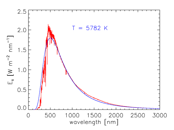
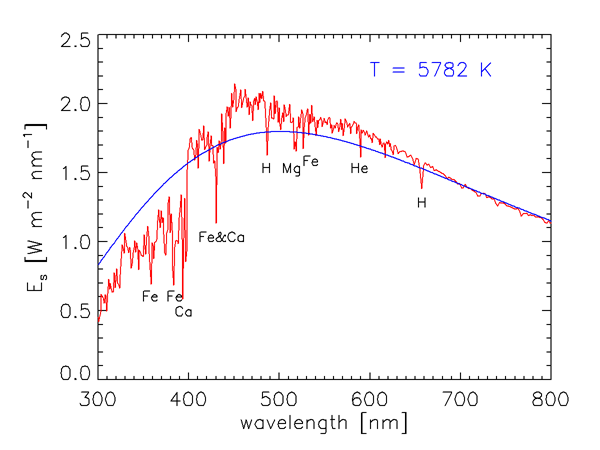
Figure 2 shows over the wavelength range of most interest in optical oceanography and ocean color remote sensing. The elements in the Sun’s atmosphere causing the most prominent Fraunhofer lines are identified. The Fraunhofer line at 587.5 nm is the line that was originally used in 1868 to deduce the existence of a new element, named Helium (after Helios, the Greek god who personified the Sun), in the Sun’s atmosphere 30 years before it was discovered on earth.
It is seldom necessary for optical oceanographers to concern themselves with the detailed wavelength dependence of seen in Fig. 2. It is usually sufficient to deal with values averaged over bandwidths of size , which correspond to the bandwidths of the optical instruments routinely used in underwater measurements and remote sensing. Table 1 gives the distribution of in several broad wavelength bands. About two thirds of the Sun’s energy is in the near-ultraviolet to near-infrared bands relevant to optical oceanography.
| Band | Wavelength Interval (nm) | Irradiance | Fraction of (percent) |
| ultraviolet and beyond | 62 | 4.5 | |
| near ultraviolet | 350-400 | 57 | 4.2 |
| visible | 400-700 | 522 | 38.2 |
| near infrared | 700-1000 | 309 | 22.6 |
| infrared and beyond | 417 | 30.5 | |
| totals | 1367 | 100.0 |
It is not the solar irradiance at the top of the atmosphere, but rather the sunlight that actually reaches the sea surface, that is relevant to oceanography. The magnitude and spectral dependence of the solar radiation reaching the earth’s surface are highly variable functions of the solar angle from the zenith (i.e., of the time of day, date, and latitude) and of atmospheric conditions (cloud cover, humidity, aerosols, ozone concentration, etc.). Figure 3 illustrates the variability in how much of the total solar irradiance reaches the sea surface. The red curve in that figure is the extraterrestrial solar irradiance averaged over 10 nm bands. The other curves show the total (diffuse plus direct) sea-level downwelling plane irradiance for a range of sun and sky conditions, also averaged over 10 nm bands. These curves were computed using an extended RADTRAN atmospheric radiative transfer model (Gregg and Carder (1990), as extended to 300 and 1000 nm).
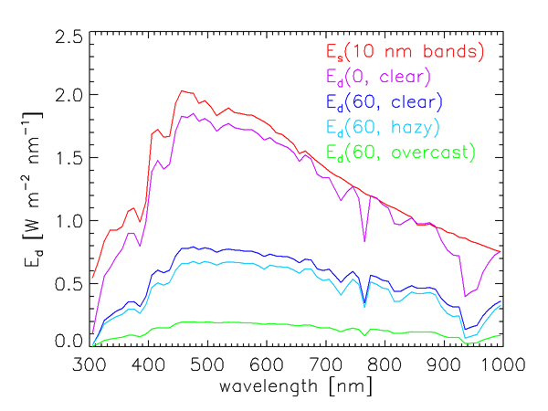
The curve in Fig. 3 is for the Sun at the zenith and a clear marine atmosphere (marine aerosols, sea-level relative humidity 80%, horizontal sea-level visibility 15 km, etc.). Rarely would this much of the solar irradiance actually reach the earth’s surface. The curve is for the same atmospheric conditions, but with the sun at a 60 deg zenith angle. The reduction in the surface irradiance is due primarily to the increased path length through the atmosphere. The curve shows the effect of going from a clear atmosphere to a cloud-free atmosphere but with increased humidity (95%) and aerosol concentration (mixed marine and continental aerosols) , leading to a hazy atmosphere with reduced visibility (5 km). The green curve is for a heavy overcast, for which no Sun is visible.
The sea-level irradiances seen in Fig. 3 also show the effects of absorption by gases in the earth’s atmosphere. Ozone (which was 300 Dobson units in these computations) greatly reduces the irradiance reaching the surface near 300 nm. The prominent dip near 765 nm is due to oxygen, and the broad dip starting near 930 nm is due to water vapor.
Table shows typical sea-level irradiances over the visible wavelength band from 400 to 700 nm. These values can show considerable variability depending on cloudiness and atmospheric conditions.
| Environment | Irradiance |
| solar irradiance above the atmosphere (for comparison) | 522 |
| very clear atmosphere, sun at the zenith | 500 |
| clear atmosphere, sun at 60 deg | 250 |
| hazy atmosphere, sun at 60 deg | 175 |
| hazy atmosphere, sun near the horizon | 50 |
| heavy overcast, sun at the zenith | 125 |
| heavy overcast, sun near the horizon | 10 |
| clear atmosphere, full moon near the zenith | |
| clear atmosphere, starlight only | |
| cloudy night | |
| clear atmosphere, light from a single, bright star | |
| clear atmosphere, light from a single, barely visible star |
Photon Calculations
It is instructive to consider the number of photons needed to generate typical irradiances and the environmental effects of these irradiances. Recall from Eq. (1) of the Units page that a single photon carries an energy of Consider a clear-sky solar irradiance of, say, , i.e., on each square meter each second. If we use for the average wavelength of the solar irradaince, this irradiance corresponds to
photons per second on every square meter of surface. Even the irradiance from the faintest star corresponds to tens of millions of photons per second per square meter.
The heating rate of the water due to absorbed irradiance is (from Eq. (6) of the Gershun’s law page)
where
- is the temperature in deg C
- is the time in seconds
- is the specific heat of sea water at constant volume
- is the density of sea water
If this irradiance is absorbed by the upper one meter of water (as can be the case in very turbid water), then the heating rate within that 1 m layer of water is
A 10 hour day at this heating rate gives an increase of , which is very large.
The linear momentum imparted to the 1 m layer of water by absorption of these photons is, by Eq. (??),
This is comparable to the linear momentum of only 1 cubic millimeter of water moving at a speed of . Thus the linear momentum transported to the ocean by incident sunlight is completely negligible compared to that transported by wind and other process that drive ocean currents.
Equation (3) of the Units page gives the maximum angular momentum that can be carried by these photons:
This is comparable to the angular momentum of a small sand grain rotating at one revolution per second. This angular momentum is much less than that of even the smallest turbulent eddies generated by current shears or breaking waves. Moreover, the maximum angular momentum computed here is transferred only of all photons are in the same angular momentum state, i.e., only if the light is 100% circularly polarized. For unpolarized light, the net transfer of angular momentum is zero (Hecht (1989)).
This we see that the physical importance of the sunlight incident on the upper ocean lies in its energy transport and not in its momentum transport. This is consistent with everyday experience: sunlight heats us up, but it does not push us around.
 See comments posted for this page and leave your own.