Ocean Color

Remote sensing of the ocean uses electromagnetic signals from the near UV (wavelengths from $\sim 300to400nm$) to various radar bands (wavelengths from $\sim 1cm$ to $\sim 1m$). This chapter discusses ocean color radiometery, commonly called ”ocean color remote sensing,” which typically uses visible (400 to 700 nm) and near-IR (wavelengths from 700 to less than 2000 nm) light. Ocean color remote sensing uses data obtained from aircraft- or satellite-borne instruments to obtain information about the constituents of natural waters, the corresponding IOPs, or the bottom depth and type.

The applications of ocean color remote sensing are extensive, varied, and fundamental to understanding and monitoring the global ecosystem. The current applications of ocean color data include

• Mapping of chlorophyll concentrations
• Measurement of inherent optical properties such as absorption and backscatter
• Determination of phytoplankton physiology, phenology, and functional groups
• Studies of ocean carbon fixation and cycling
• Monitoring of ecosystem changes resulting from climate change
• Fisheries management
• Mapping of coral reefs, sea grass beds, and kelp forests
• Mapping of shallow-water bathymetry and bottom type for military operations
• Monitoring of water quality for recreation
• Detection of harmful algal blooms and pollution events

The International Ocean Colour Coordinating Group (IOCCG) has a lengthy report, Why Ocean Colour? The Societal Benefits of Ocean-Colour Technology describing the many applications and societal benefits or ocean color remote sensing. A National Research Council study Assessing the Requirements for Sustained Ocean Color Research and Operations also shows the diversity of ocean color applications. These reports give many additional applications and details about each.

Remote sensing can be active or passive. Active remote sensing means that a signal of known characteristics is sent from the sensor platform—an aircraft or satellite—to the ocean, and the return signal is then detected after a time delay determined by the distance from the platform to the ocean and by the speed of light. One example of active remote sensing at visible wavelengths is the use of laser-induced fluorescence to detect chlorophyll, yellow matter, or pollutants. In laser fluorosensing, a pulse of UV light is sent to the ocean surface, and the spectral character and strength of the induced fluorescence at UV and visible wavelengths gives information about the location, type and concentration of fluorescing substances in the water body. Another example of active remote sensing is lidar bathymetry. This refers to the use of pulsed lasers to send a beam of short duration, typically about an nanosecond, toward the ocean. The laser light reflected from the sea surface and then slightly later from the bottom is used to deduce the bottom depth. The depth is simply $0.5\left(c∕n\right)\Delta t$, where $c$ is the speed of light in vacuo, $n$ is the water index of refraction, $\Delta t$ is the time between the arrival of the surface-reflected light and the light reflected by the bottom, and the 0.5 accounts for the light traveling from the surface to the bottom and back to the surface. Laser fluorosensing and lidar bathymetry are discussed in detail in Measures (1992).

In passive remote sensing we simply observe the light that is naturally emitted or reflected by the water body. The night-time detection of bioluminescence from aircraft is an example of the use of emitted light at visible wavelengths. The most common example of passive remote sensing, and the one primarily discussed in this chapter, is the use of sunlight that has been scattered upward within the water and returned to the sensor. This light can be used to deduce the concentrations of chlorophyll, CDOM, or mineral particles within the near-surface water; the bottom depth and type in shallow waters; and other ecosystem information such as net primary production, phytoplankton functional groups, or phytoplankton physiological state.

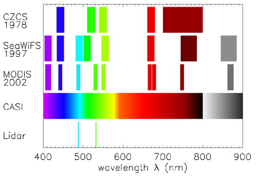
Passive ocean color remote sensing from satellites began with the the Coastal Zone Color Scanner (CZCS), which was launched in 1978. CZCS was a multi-spectral sensor, meaning that it had only a few wavelength bands with bandwidths of 10 nm or more. After the phenomenal success of that “proof of principle” sensor, numerous other multispectral sensors have been developed and launched. Those later sensors generally had a few more bands with narrower bandwidths. Thus the Sea-viewing Wide Field-of-view Sensor (SeaWiFS) added a band near 412 nm to improve the detection of CDOM. The near-IR bands are used for atmospheric correction. There is today much interest in the use of hyperspectral sensors, which typically have 100 or more bands with nominal bandwidths of 5 nm or less. Figure 1 shows the wavelength bands for a few representative sensors. The MODIS (MODerate resolution Imaging Spectroradiometer) sensor has additional bands in the 400-900 nm range, not shown in Fig. 1, which are used for detection of clouds, aerosols, and atmospheric water vapor. The bands shown are the ones used for remote sensing of water bodies. The launch dates of the three satellite sensors are shown. The Compact Airborne Hyperspectral Imager (CASI) is a commercially available hyperspectral sensor that is widely used in airborne remote sensing of coastal waters. It has 228 slightly overlapping bands, each with a nominal 1.9 nm bandwidth and covering the 400 - 1000 nm range. CASI users often select a subset of these bands as needed for a particular application. Lidar bathymetry systems typically use either 488 nm in “blue” water or 532 nm in “green” water. Those wavelengths can be obtained from high-power lasers and give close to optimum water penetration for the respective water types.

Although remote sensing usually obtains information for one spatial point at a time, most applications combine measurements from many points to build up an image, i.e. a 2D spatial map of the ocean displaying the desired information at a give time. Imagery acquired at different times then gives temporal information. Satellite systems typically have spatial resolution (the size of one image pixel at the ocean surface) of 250 m to 1 km. Those systems are useful for regional to global scale studies. Airborne systems can have resolutions as small as 1 m, as required for applications such as mapping coral reefs.

Passive ocean-color remote sensing is conceptually simple. Sunlight, whose spectral properties are known, enters the water body. The spectral character of the sunlight is then altered, depending on the absorption and scattering properties of the water body, which of course depend on the types and concentrations of the various constituents of the particular water body. Part of the altered sunlight eventually makes its way back out of the water and is detected by the sensor on board an aircraft or satellite. If we know how different substances alter sunlight, for example by wavelength-dependent absorption, scattering, or fluorescence, then we can hope to deduce from the altered sunlight what substances must have been present in the water, and in what concentrations. However, this process of “working backwards” from the sensor to the ocean is an inverse problem that is fraught with difficulties, as seen on the next pages. Nevertheless, these difficulties can be overcome, and ocean color remote sensing has completely revolutionized our understanding of the oceans at local to global spatial scales and daily to decadal temporal scales.