Wave Variance Spectra: Examples

This page gives two examples of wave elevation variance spectra. The Pierson-Moskowitz omnidirectional spectrum describes gravity waves in a “fully developed” sea. A fully developed sea is an idealization of the statistically steady-state wave field resulting from a steady wind blowing for an infinitely long time over an infinite fetch. (In practice, the duration and fetch required to achieve something close to a fully developed sea depend on the wind speed. A steady wind of $5m{s}^{-1}$ blowing for 10 hours over a fetch of 60 km might be adequate; for hurricane winds of $35m{s}^{-1}$, a fetch of a few thousand kilometers and a duration of several days would be required. Thus it is much easier to approach a fully developed sea at low wind speeds than at high.)

The Elfouhaily et al. directional spectrum includes both gravity and capillary waves scales. Moreover, it has a parameter that describes the wave age, so than any sea state from young (the wind has just started blowing) to fully developed can be simulated. The Elfouhaily et al. spectrum will be used to generate the two-dimensional sea surface examples on the following pages.

The Pierson-Moskowitz Omnidirectional Gravity Wave Spectrum

The omnidirectional Pierson and Moskowitz (1964) spectrum, formulated in terms of angular spatial frequency $k$, is

where

$\alpha =0.0081$,

$\beta =0.74$,

$g=9.82m{s}^{-2}$ is the acceleration of gravity,

$U_{19}$ is the wind speed in $m{s}^{-1}$ at 19.5 m above the sea surface, and

$k$ is the angular spatial frequency in $rad{m}^{-1}$.

The wind speed at 19.5 m can be obtained from the more commonly used wind at 10 m above the sea surface by the approximate formula

As has already been noted, it is often of interest to express a variance spectrum in terms of other variables, such as the wavenumber $\nu$ or the temporal angular frequency $\omega$. To change variables in a spectral density function, the key is to recall that a variance density function by definition expresses the variance per unit frequency interval. The variance contained in some interval $dk$ of the spatial angular frequency equals the variance contained in the corresponding interval $d\nu$ of the wavenumber or the interval $d\omega$ of the temporal frequency. Thus we have

To change the variable from $k=2\pi \nu$ to $\nu$, the previous equation gives

which results in

To change variables from spatial angular frequency $k$ to temporal angular frequency $\omega$, we use the dispersion relation for gravity waves in deep water,

to evaluate

which leads to

All of these formulas have units of meters squared over the appropriate frequency. (The quantities $dk∕d\nu$ and $dk∕d\omega$ seen in the conversions are the Jacobians for the one-dimensional changes of variables.) Figure 1 shows the Pierson-Moskowitz spectrum as functions of $k$ and $\omega$ for wind speeds of $U_{10}=5,10$, and $15m{s}^{-1}$.

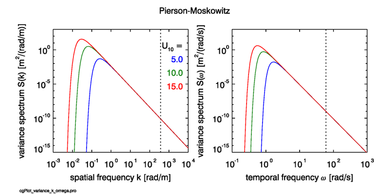
This spectrum has withstood the test of time fairly well (Alves and Banner (2003)) as a description of gravity waves in fully developed seas. However, it should not be used for high-frequency (short-wavelength) gravity waves, and certainly not for capillary waves. Likewise, it does not describe young seas, which have not had the time or fetch needed to approach the state of a well developed sea.

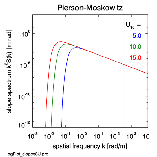
Figure 2 shows the Pierson-Moskowitz slope spectra for three wind speeds. Note that the slope spectrum falls off much more slowly for high frequencies than does the elevation spectrum. That means that the higher frequencies contribute much more to the total slope variance than they do to the total elevation variance.

The Elfouhaily et al. Directional Gravity-Capillary Wave Spectrum

In order to model two-dimensional sea surfaces $z\left(x,y\right)$, we need a 2-D wave elevation variance spectrum that describes the distribution of wave variance for waves propagating in difference directions. The numerical examples of 2-D sea surfaces to be seen on the following pages use the 2-D elevation variance spectrum of Elfouhaily et al. (1997), which is described here for later reference. For brevity, this paper and their model are denoted here by “ECKV,” taken from the initials of the authors’ last names.

The ECKV spectrum has an omnidirectional variance spectrum that explicitly includes both the gravity and capillary wave scales. The boundary between gravity and capillary waves is taken to be $k=\sqrt{\rho g∕\tau }=370rad∕m$, the angular spatial frequency at which the restoring forces (which tend to bring a wave surface back to an unperturbed level surface) of gravity and surface tension are equal. The corresponding wavelength is $\Lambda =2\pi ∕370=0.017m$. ECKV then combine their omnidirectional spectrum with a spreading function to obtain their one-sided, directional variance spectrum. Using their notation, the 2-D ECKV spectrum has the form

Here $\mathcal{𝒮}\left(k\right)$ is the 1-D omnidirectional spectrum with units of $m^2∕\left(rad∕m\right)$, and $\Phi \left(k,\phi \right)$ is a non-dimensional spreading function. $\Psi \left(k,\phi \right)$ thus has units of $m^2∕{\left(rad∕m\right)}^2$. Equation labels such as [ECKV 45] give for reference the corresponding equation in the ECKV paper.

The ECKV omnidirectional spectrum is

where $B_l$ is the low-frequency (long gravity wave) contribution to the variance, and $B_h$ is the high-frequency (short gravity wave to capillary wave) contribution. (The quantity $k^3\mathcal{𝒮}\left(k\right)$ is called the curvature or saturation spectrum and is of interest in physical oceanography because it is related to the rate of variance dissipation of the waves. Thus ECKV refer to $B_l$ and $B_h$ as the low and high frequency curvature spectra.) The components of the omnidirectional spectrum are given by

where

$\alpha =0.0081$,

$\beta =1.25$,

$g=9.82m{s}^{-2}$ is the acceleration of gravity,

$U_{10}$ is the wind speed in $m{s}^{-1}$ at 10 m above the sea surface

$k$ is the angular spatial frequency in $rad{m}^{-1}$

${\Omega }_c$ is defines the age of the waves for the given wind speed:

= 0.84 for a fully developed sea (corresponds to Pierson-Moskowitz)

= 1 for a “mature” sea [used in ECKV Fig 8a]

= 2 to 5 for a “young” sea; the maximum allowed value is 5

$C{d}_{10N}=0.00144$ is a drag coefficient [value deduced from ECKV Fig 11]

$u^{\ast }=\sqrt{C{d}_{10N}}{U}_{10}$ is the friction velocity [using ECKV 61]

$a_o=0.1733$ (ECKV 59)

$a_p=4.0$

$k_m=370.0rad∕m$

$c_m=0.23m∕s$ is the phase speed of the wave with spatial frequency $k_m$

$a_m=0.13u^{\ast }∕c_m$ [ECKV 59]

$\gamma =1.7if{\Omega }_c\le 1else\gamma =1.7+6{log}_{10}\left({\Omega }_c\right)$

$\sigma =0.08\left(1+4{\Omega }_c^{-3}\right)$

${\alpha }_p=0.006{\Omega }_c^{0.55}$ [ECKV Eq. 34]

${\alpha }_m=0.01\left[1+ln\left(u^{\ast }∕c_m\right)\right]if{u}^{\ast }\le c_{m}else{\alpha }_m=0.01\left[1+3ln\left(u^{\ast }∕c_m\right)\right]$ [ECKV 44]

$k_o=g∕U_{10}^2$

$k_p=k_o{\Omega }_c^2$ is the spatial frequency of the maximum of the spectrum

$c_p=\sqrt{g∕k_p}$ is the phase speed of the wave with spatial frequency $k_p$

$c=\sqrt{\left(g∕k\right)\left(1+{\left(k∕k_m\right)}^2\right)}$ is the phase speed of the wave

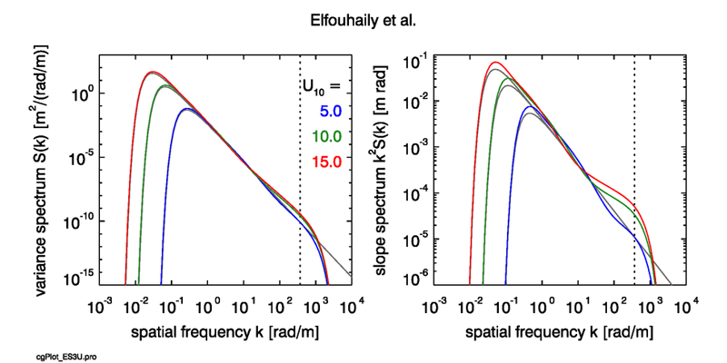
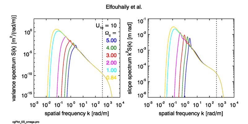
At the lower frequencies, the ECKV spectrum is essentially the Pierson-Moskowitz spectrum (the $L_{PM}$ term above) with an enhancement (the $J_p$ term) that adds more energy to the lower frequencies. The highest frequencies have a cutoff due to viscous damping of the smallest capillary waves. The ECKV omnidirectional elevation and slope spectra are illustrated in Fig. 3 for the case of a fully developed sea and three wind speeds. Figure 4 shows the spectra as a function of wave age for a wind speed of $U_{10}=10m{s}^{-1}$.

Spreading Functions

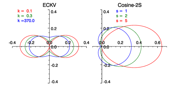
The ECKV spreading function is given by

Note that this function is symmetric about $\phi =\pi ∕2$; i.e., the function has symmetric spreading downwind and upwind. This is consistent with a symmetric variance spectrum $\Psi \left(-k\right)=\Psi \left(k\right)$ as would be obtained from the Fourier transform of a snapshot of a sea surface. This symmetry will be explained on the following pages.

A commonly used family of alternate spreading functions is given by the “cosine-2s” functions of Longuet-Higgins et al. 1963, which have the form

where the normalizing coefficient is

and $s$ is a spreading parameter that in general depends on $k$, $U_{10}$, and wave age. In this equation $\Gamma$ is the customary gamma function defined by $\Gamma \left(p\right)\equiv {\int \; <!--nolimits-->}_0^{\infty }{x}^{p-1}{e}^{-x}dx$ where $p>0$. The cosine-2s functions are asymmetric, with much stronger downwind than upwind propagation.

The ECKV and cosine-2s spreading functions are illustrated in Fig. 5. Both of these functions satisfy the normalization condition (??). Both spreading functions transition from strongly forward peaked at low spatial frequencies (long gravity waves; the red curves) to curves with significant propagation at right angles to the wind at high frequencies (capillary waves; the blue curves). The cosine-2s curves are asymmetric in $\pm k$ and have at least a small amount of upwind propagation at all frequencies (except at exactly upwind, $\phi =\pi$). Not surprisingly, the real ocean is more complicated than either of these models. In particular, observations of long-wave gravity waves tend to show a bimodal spreading about the downwind direction, which transitions to a more isotropic, unimodal spreading at shorter wavelengths (Heron (2006). However, the simple models of Eqs. (6) and (7) are adequate for the present purpose of illustrating surface-generation techniques. The effect of the choice of spreading function on the generated waves will be illustrated on the Spreading Function Effects page.

On the following pages we will learn the important distinction between “one-sided” or “folded” spectra and the associated “two-sided” spectra. The ECKV spectrum as given above is a one-sided spectrum.