Cox-Munk Sea Surface Slope Statistics

The Cox-Munk Sea Surface Slope Statistics

Cox and Munk (1954a) and Cox and Munk (1954b) analyzed aerial photographs of the Sun’s glitter patterns on wind-blown sea surfaces, from which they were able to deduce the slope statistics of the sea surface as a function of the wind speed. (See also Cox and Munk (1955).) Figure 1 shows one such photograph. The wind speed, measured from a ship within the area photographed, was 4.6 m/s.

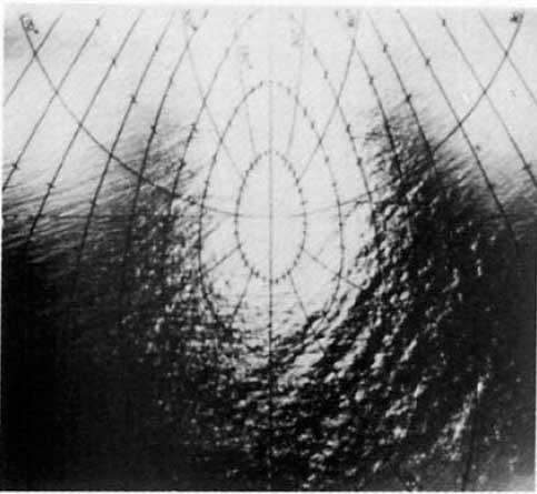
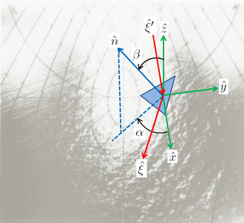
If the surface were perfectly flat (i.e., zero wind speed and no swell) and the sky were black, the glitter pattern would be a single bright spot at the Sun’s specular reflection direction, which is at the center of the photograph. However, wind ruffles the sea surface so that the Sun’s direct beam can be reflected from a wider area of the sea surface into the observer’s direction. In order for a wave facet to reflect a solar ray towards the observer, the facet must be tilted in just the right way so that the tilted facet can reflect an incident ray from the Sun into the direction of the observer. This is illustrated in Fig. 2. The blue triangle represents a tilted wave facet that is reflecting an incident solar ray ${\widehat{\xi }}^{\prime }$ into the observer’s direction $\widehat{\xi }$. The $\left(\widehat{x},ŷ,ẑ\right)$ coordinate system shown by the green arrows is a Sun-centered system with $-\widehat{x}$ pointing horizontally towards the Sun, $ẑ$ vertically upward (normal to the mean sea surface), and $ŷ=ẑ\times \widehat{x}$. The Sun’s incindent ray ${\widehat{\xi }}^{\prime }=\left({\xi }_x^{\prime },{\xi }_y^{\prime },{\xi }_z^{\prime }\right)$ thus has ${\xi }_x^{\prime }>0$, ${\xi }_y^{\prime }=0$, and ${\xi }_z^{\prime }<0$. $\widehat{n}$ is the normal to the tilted facet. Polar angle $\beta ={cos}^{-1}\left(\widehat{n}\cdot ẑ\right)$ measures the tilt of the facet from the normal to the mean sea surface. Azimuthal angle $\alpha$ measures the orientation of the facet relative to the $\widehat{x}$ axis, with $\alpha$ being measured clockwise from $\widehat{x}$ as shown.

[Comment: The analysis of the glint photographs requires several coordinate systems. One is Sun-centered, as seen in Fig. 2. Another system is used to define the image plane of the camera recording the glitter patterns. Use of the surface statistics to be presented below for generation of random realizations of wind-blown surfaces requires a wind-centered system $\left(î,ĵ,\widehat{k}\right)$, with $î$ pointing downwind, $ĵ$ cross-wind, and $\widehat{k}=ẑ$. Figure 2 shows the $\left(\widehat{x},ŷ,ẑ\right)$ system as used in Preisendorfer and Mobley. The Sun system used in the Cox and Munk papers has $ŷ$ pointing horizontally toward the Sun, with $\alpha$ measured from $ŷ$ “to the right of the Sun.” Conversion from one system to the other is straightforward but tedious trigonometry; the details are given in Section 7(a) of Preisendorfer and Mobley (1985) and inPreisendorfer and Mobley (1986) . Fortunately, these details do not concern us here.]

Let $\eta \left(x_a,x_c\right)$ be the sea surface elevation in a wind-centered coordinate system where $x_a$ is in the along-wind direction (with $x_a$ positive in the downwind or $î$ direction) and $x_c$ is in the cross-wind direction (with $x_c$ positive in the $ĵ$ direction). Then

are respectively the sea surface slopes in the along-wind and cross-wind directions. After laborious analysis of numerous photographs for different solar zenith angles and wind speeds, Cox and Munk found that the statistical distribution of the random sea surface slopes ${\eta }_a$ and ${\eta }_c$ is, to a good approximation, a bivariate Gaussian:

where ${\sigma }_a^2$ and ${\sigma }_c^2$ are respectively the variances of the slopes in the along-wind and cross-wind directions. Note that $p\left({\eta }_a,{\eta }_c\right)$ is normalized as required for a probability distribution function, i.e.,

These slope variances were found to be related to the wind speed $U$ in meters per second at “mast height” (41 feet or 12.5 m) by

Equations 1-4 are the celebrated Cox-Munk wind speed-wave slope statistics. The non-zero value of ${\sigma }_c^2$ at zero wind speed results from a residual amount of slope that is not attributable to the local wind. This contribution to ${\sigma }_c^2$ is often ignored when modeling sea surfaces, so that a wind speed of zero corresponds to an exactly flat sea surface.

Duntley (1954) used closely spaced vertical wires to measure surface elevations at the two wires, from which the slope could be obtained. His measurements were consistent with the values obtained by Cox and Munk. Several later studies have found some dependence on the air-sea temperature difference, i.e., on the atmospheric stability, although sometimes with conflicting conclusions, perhaps because the sea states were not in a mature state for the given wind speed. The slope variances are also sensitive to the presence of films (e.g., from oil) that tend to dampen waves, especially at the smallest spatial scales. Cox and Munk themselves did measurements within areas where they had poured a mixture of oils onto the sea surface; those values are found in the papers cited. Regardless of potential improvements to the Cox and Munk values, the original values of the slope variances are widely used, e.g. they are one option for surface generation in the HydroLight radiative transfer code, and they are used by NASA for atmospheric correction. The numerous successful applications of the Cox-Munk equations have proven that their values are sufficiently accurate for a wide range of conditions.

It should be noted that the Cox-Munk statistics are based on observations, so they describe the slope effects of whatever waves were on the sea surface at the times the photographs were taken. They thus describe the full range of long-wavelength gravity to short-wavelength capillary waves for the sea states at the time of observation. Note, indeed, the obvious presence of long-wave swell at the lower right of Fig. 1. It is often stated (e.g., in Preisendorfer and Mobley (1985) and in Section 4.3 of Light and Water (1985)) that these slope statistics refer to capillary waves, which is incorrect. Capillary waves are responsible for much of the slope variance, and they are included in the Cox-Munk statistics, but the gravity waves are also included.

Sea Surface Simulations

Preisendorfer and Mobley (1985) and (1986) showed how to use the Cox-Munk statistics to generate random realizations of wind-blown sea surfaces (see also Section 4.3 of Light and Water (1994)). The mathematical details need not be repeated here, but the procedure is as follows. First, they divide a hexagonal patch of sea surface into triangluar wave facets. Then the Cox-Munk along-wind and cross-wind variances are used in conjunction with a random number generator to define, for a given wind speed, the relative surface elevations at the vertices of the triangular wave facets. The slopes of the resulting surface facets then reproduce, on average, the slope statistics of a real sea surface. Figure 3 shows an example of such a surface realization for a wind speed of 10 m/s. These Cox-Munk surfaces are “scale independent.” That is, only the slopes matter, not the actual physical size of the patch of surface. Thus no units are shown for the axes. Note that, in this figure, the vertical scale (the surface elevations) is greatly expanded relative to the horizontal scales (the x axis is the along-wind direction, and the y axis is the cross-wind direction).

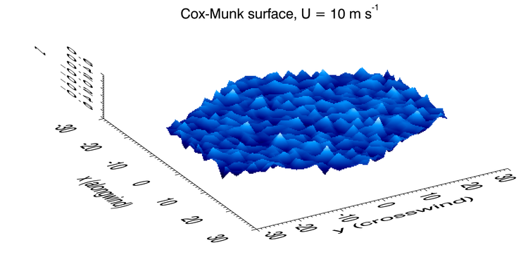
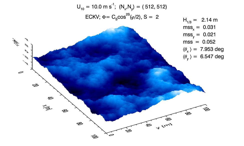
This technique does not reproduce the sea surface elevation statistics of a real sea surface. Although the surface realization seen in Fig. 3 correctly reproduces the Cox-Munk slope variances, it simply does not look like a real sea surface. In particular, there is no spatial correlation from one point on the surface to another nearby point, as occurs with real water waves. However, both the elevation and slope statistics can be reproduced using more advanced techniques, which are described in the Level 2 material of this chapter, starting at Modeling Sea Surfaces. Those techniques are based on sea surface elevation variance spectra and use fast Fourier transforms (FFTs); Here, surfaces generated by these techniques will be called FFT surfaces for brevity. Figure 4 shows an example surface constructed using the techniques of Level 2. The inset shows the mean square slopes in the along-wind ($ms{s}_x$) and cross-wind ($ms{s}_y)$ directions; these values correspond to ${\sigma }_a^2$ and ${\sigma }_c^2$, respectively, in the Cox-Munk equations. For a wind speed of $10m{s}^{-1}$, the Cox-Munk equations give ${\sigma }_a^2=0.0316$ and ${\sigma }_c^2=0.0222$, which agree well with the values shown in the figure for this particular FFT surface realization. The value $H_{1∕3}=2.14m$ is the significant wave height, which is in agreement with the wave heights for a mature sea at this wind speed. Note that the figure axes are now in meters, because an actual $100\times 100$ meter patch of sea surface is being simulated, although the scale of the vertical axis is still exaggerated compared to the horizonal scales.

Optical Differences in Sea Surfaces

The obvious next question is this: How much do optical quantities such as the sea surface reflectance or water-leaving radiance differ for a Cox-Munk surface like that of Fig. 3 versus a more realistic FFT surface like that of Fig. 4? This can be answered by Monte Carlo simulation. In such simulations, a large number (often millions) of random sea surface realizations are generated. For each surface, rays simulating the Sun and sky incident radiance are sent toward the surface, where they are reflected and transmitted by the surface wave facets according to the Fresnel equations applied to the point where a ray intersects a wave facet. In this manner, the reflected and transmitted radiances are built up ray by ray. The mathematical details of these computations are rather ugly; see Preisendorfer and Mobley (1985) or Appendix B of Mobley (2014) for a detailed description of a ray tracing algorithm that fully accounts for the possibility of multiple scattering between wave facets.

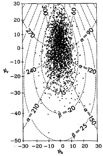
Figure 5 shows an example of a simulated solar glitter pattern created by ray tracing and a Cox-Munk surface. In this figure, the final direction of each ray is plotted as a dot where the ray intersects the image plane of a camera photographing the glitter pattern from the air. The pattern of this simulated glitter pattern should be compared with central glitter pattern of Fig. 1. The two patterns are in qualitative agreement.

A feeling for the optical differences of various sea surfaces can be obtained by comparison of their surface-reflected radiances, i.e., their glitter patterns. The left panel of Fig. 6 shows the surface-reflected radiance for a Cox-Munk surface and a wind speed of $5m{s}^{-1}$, as generated by HydroLight. The Sun was at a zenith angle of 50 deg in a clear sky. The Sun’s azimuthal angle was in the down-wind direction (the arrow at the middle of the plot indicates the wind direction). The water IOPs were based on an albedo of single scattering of 0.8 and the sky conditions were for a wavelength of 550 nm. The ray tracing that underlies these calculations used 250,000 sea surface realizations; there is a negligible amount of Monte Carlo noise in these results. The colors display contours of the radiance, with the lightest color being the highest radiance; the contour spacing is not linear but was chosen for visual effect. The light colored area at the right of the polar plot is the glitter pattern as would be seen by an observer looking downward at the sea surface and facing the sun at an azimuthal viewing angle of ${\phi }_v=0$. The concentric circles show off-nadir viewing angles of 30, 60, and 90 deg (the horizon). The radiance is largest near the horizon, rather than near the specular direction, because of the large increase in the Fresnel reflectance for angles of reflection greater than about 60 deg. The right panel of the figure shows the glitter pattern for an FFT surface, with all else being the same.

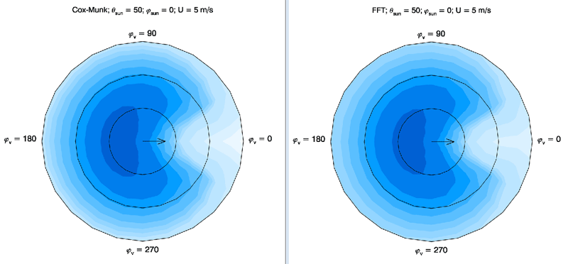
Some differences in the glitter patterns can be seen in the contour plots of Fig. 6, but a more quantitative comparison can be made by plotting the radiances as a function of polar angle in the plane of the Sun. This is done in Fig. 7, using the data of Fig. 6. This plot shows that for viewing directions out to about 60 deg in the azimuthal direction of the Sun, there is only a few percent difference in the surface-reflected radiances. For viewing directions near the horizon, the difference increases to several tens of percent, with the Cox-Munk surface having the ”brighter” glitter pattern near the horizon.

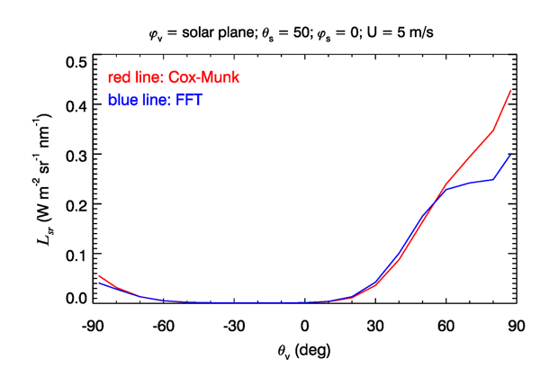
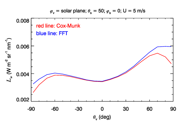
Figure 8 shows the corresponding water-leaving radiances, which determine the remote-sensing reflectance. Again, there is very little difference (at most a few percent) for off-nadir viewing directions less than about 50 deg, which covers the range of most ocean-color remote sensing. However, for viewing directions near the horizon, the difference in the Cox-Munk and the FFT surface is again a few tens of percent.

The details of these comparisons will be different for different Sun zenith angles and different wind speeds. However, it is generally true that the sea surface affects the water-leaving radiance by only a few percent for the near-nadir viewing directions relevant to most remote sensing. Surface effects are most prominent in the glitter patterns themselves. There are also differences when the Sun is in the along-wind versus the cross-wind direction. However, a full discussion of such matters is a topic for elsewhere.