Page updated:
April 14, 2021
Author: Curtis Mobley
View PDF
A New IOP Model for Case 1 Water
This page develops a new IOP model for Case 1 water based on recent publications on absorption and scattering in Case 1 waters. The genesis of this model was to have an IOP model that made use of the latest data (at the time of its creation) and was convenient for use in the HydroLight radiative transfer model, where it can be selected as the “New Case 1 IOP Model”. In this model all IOPs are determined by the chlorophyll value (after selecting low, medium, or high ultraviolet absorption). This model is presumably an improvement over previous models, although that remains to be proven by comparison with comprehensive measurements. In any case, the inherent limitations of IOP models must be remembered (in particular, see Mobley et al. (2004) for limitations of the “Case 1” concept). IOP models may be very good on average, but may or may not be (very often, definitely are not) correct in any particular instance. IOP models are therefore best used for “generic” studies. When modeling a particular water body, especially in a closure study, it is always best to use measured data to the greatest extent possible.
Particle absorption
.
It is well known that there is great variability in chlorophyll-specific absorption spectra . In particular, the spectral shape of changes with the chlorophyll concentration, owing to species composition and pigment packaging effects (e.g., Bricaud et al. (1995), Bricaud et al. (1998)). Thus the next step in improving the particle absorption model is to allow the chlorophyll-specific absorption to depend on the chlorophyll concentration itself. Bricaud et al. (1998) therefore model particle absorption as
The Bricaud et al. (1998) paper gives and between 400 and 700 nm. Extending the Bricaud et al. values from 700 to 1000 nm is easy because phytoplankton absorption is essentially zero in the infrared (IR). However, there are very few measurements of phytoplankton absorption below 350 nm, so extending and down to 300 nm is at best an uncertain process.
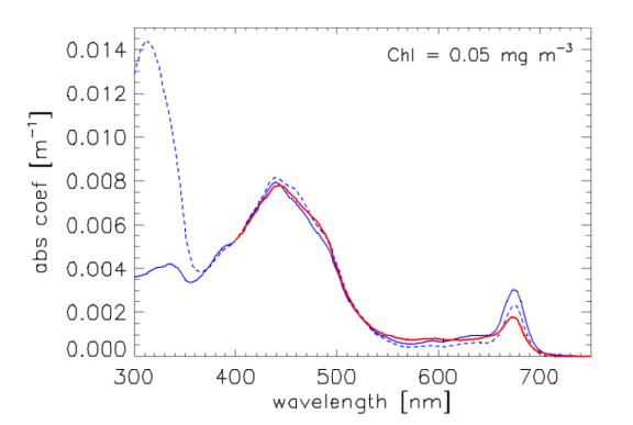
Morrison and Nelson (2004) [their Fig. 1] show two normalized phytoplankton absorption spectra from 300 to 750 nm taken at the Bermuda Atlantic Time Series (BATS) site. The BATS Chl values ranged between 0.002 and over the course of a year, with a mean of 0.152. Although their spectra are similar above 365 nm, they are highly variable with season and depth between 300 and 365 nm. This variability is likely due to mycosporine-like amino acids (MAAs), which strongly absorb near 320 nm. Figure 1 compares the Morrison and Nelson spectra (blue curves) with the Bricaud et al. of Eq. (1) evaluated for (red curve); the Morrison and Nelson spectra are normalized to the Bricaud value of . The shapes of the Morrison and Nelson spectra are consistent with the Bricaud values for low Chl values.
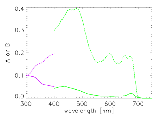
Vasilkov et al. (2005) present spectra for and and between 300 and 400 nm, as derived from absorption measurements in coastal California waters. Figure 2 shows their and spectra compared with those of Bricaud et al. (1998). The differences at 400 nm reflect the different databases (i.e., different waters) used to derive the coefficients.
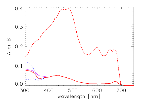
Desperation is the mother of modeling (you can quote me on that), so to define and over the 300-1000 nm range, I proceeded as follows. The Bricaud et al. A and B curves are accepted for use from 400 to 720 nm, with A = B = 0 between 720 and 1000 nm. The Vasilkov et al. curve for A was normalized to the Bricaud value at 400 nm, i.e., , where subscripts v and b stand for Vasilkov et al. and Bricaud et al., respectively. The normalized was then averaged with the two normalized spectra of Morrison and Nelson seen in Fig. 1, assuming that the A spectra have the same shape as . This assumption about the shapes of A and is correct only if B = 0 or if Chl = 1, in which case in Eq. (1). The resulting average A between 300 and 400 nm then merges smoothly with the A of Bricaud at 400 nm. For B, the Vasilkov et al. curve was normalized to the Bricaud et al. curve at 400, and the result was used to extend the Bricaud et al. B down to 300 nm. The resulting A and B spectra are shown in red in Fig. 3, along with the three A spectra used to compute the average A between 300 and 400. These A and B give an absorption model that roughly corresponds to the mid-range of UV absorptions seen in the Morrison and Nelson data. The new Case 1 IOP model uses these A and E = 1 - B as the default spectra for the last version of Eq. (1). The tabulated A and E spectra are on file AEmidUVabs.txt.
It would be interesting to compare light fields for the wide range of UV absorptions illustrated by the Morrison and Nelson spectra of Fig. 3. A spectra for low and high UV absorptions are therefore defined by simply using the shapes of the Morrison and Nelson spectra absorption spectra to extend the Bricaud A from 400 down to 300 nm. The B spectra were taken to be the same as for the mid-range of UV absorption just discussed. The spectra are on files AElowUVabs.txt (low UV absorption) and AEhighUVabs.txt (high UV absorption).
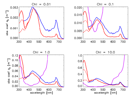
Regardless of which set of A and E spectra is chosen, the A and E spectra are used in the same manner in Eq. (1) to define for any Chl value. Figure 4 shows the resulting particle absorption spectra for low, medium, and high UV absorptions and for , and . The corresponding absorption coefficients as computed by the classic Case 1 IOP model are shown for comparison, as is absorption by pure water. There are significant differences in the classic and new models, which will lead to significant differences in computed radiances, irradiances, and AOPs when used in radiative transfer calculations. Note in particular that the shape of the particle absorption spectrum now changes with the chlorophyll value. Presumably the new model gives a more realistic description, on average, of particle absorption in Case 1 waters than does the classic model for which the shape of the particle absorption spectrum is independent of the chlorophyll concentration.
CDOM absorption
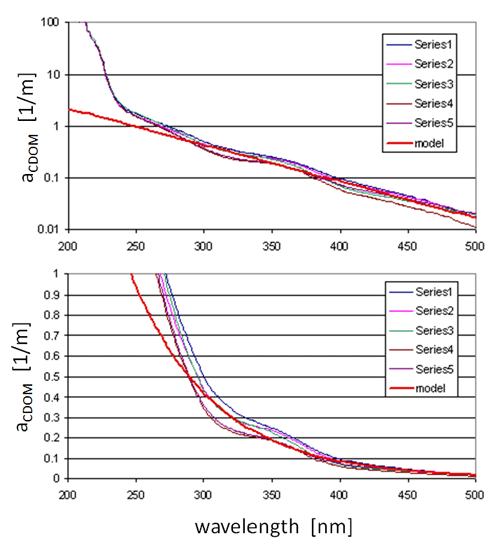
Figure 5 shows measured CDOM absorption spectra down to 200 nm at several locations in Florida waters on both log and linear ordinates. For wavelengths greater than 300 nm, these spectra are acceptably well modeled by a function of the form
| (2) |
The red line in Fig. 5 shows the spectrum predicted by Eq. (2) with , and the average (for the spectra shown) of . This value of S was determined from the average values of at 300 and 440 nm. The functional form (2) is used to model CDOM absorption down to 300 nm. This model underestimates CDOM absorption at shorter wavelengths and therefore should not be used below 300 nm. When incorporated into the new Case 1 IOP model, is set to , with default values of , , and just as in the classic Case 1 model. However, other values of , , and S can be used if desired.
Scattering
Just as for absorption, recent papers have presented improved models for particle scattering in Case 1 waters. Morel et al. (2002) (their Eq. 14) model the particle scattering coefficient as
| (3) |
where
Equation (3) with is the “classic” scattering model proposed by Gordon and Morel (1983). The wavelength dependence of the new scattering coefficient now depends on the chlorophyll concentration. In particular, now lies between -1 and 0. A value of , as often used in earlier models, is known from Mie theory to be valid only for nonabsorbing particles with a Junge particle size distribution slope of -4.
Loisel and Morel (1998) studied the relationship between particle beam attenuation at 660 nm, , and the chlorophyll concentration. They found the functional form
| (5) |
The values of and are different for near-surface (down to one “penetration depth,” as relevant to remote sensing) and deeper waters. Because at 660, Morel et al. (2002) adopt the coefficients for Eq. (5) for use in Eq. (3), after shifting the reference wavelength to 550 nm. Thus for near-surface waters, Morel et al. (2002) use = 0.416 and n = 0.766 in Eq. (5).
However, a power law in wavelength of the form of Eq. (5) generally gives a better fit for than for (e.g., Voss (1992); Boss et al. (2001c) ). Thus it is probably better to model and then obtain from (with being determined by Eq. (1) as described above). This is the approach taken in the new Case 1 model, which uses
| (6) |
where the coefficients are the same as for b in Eq. (3) above and is given by Eq. (4). Thus this model uses the chlorophyll-dependence of from Loisel and Morel (1998), Eq. :loiselcp, and assumes that has the same chlorophyll-dependent wavelength dependence as the model of Morel et al. (2002), Eq. (3) The default values of and n , which apply to near-surface waters, are = 0.407 and n = 0.795 (from Loisel and Morel, 1998, their Eq. 5); other values can be used if desired.
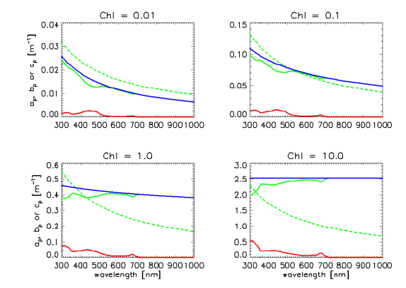
Figure 6 shows example for mid-range UV absorption, , and spectra for near-surface waters ( = 0.416 and n = 0.766 in Eq. 5), along with the ”classic” with = 0.3, n = 0.62, and m = 1. The scattering coefficients are not too different at low chlorophyll values, but the new has a different wavelength dependence and is much larger in magnitude, by up to a factor of three, at high Chl values. Unlike in the classic scattering model, the wavelength dependence of now depends on Chl and is more complicated. These differences in scattering will have a significant effect on computed radiances.
Scattering phase function
Morel et al. (2002) also developed a phase function model for Case 1 water in which the phase function is a combination of “small” and “large” particle phase functions, with the fraction of each being determined by the chlorophyll concentration:
| (7) |
where
| (8) |
Figure 9 shows phase functions determined by Eqs. (7) and (8), along with the frequently used Petzold average-particle phase function
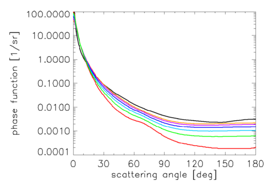
It should be noted that the Morel et al. (2002) phase functions have smaller backscatter fractions ( = 0.014 for the small particles to 0.0019 for the large particles) than the Petzold phase function ( = 0.018). This is consistent with what is known about the phase functions for algal particles (e.g., Ulloa et al. (1994), or Twardowski et al. (2001)). The Morel phase functions of Eq. (7) and Fig. 7 are adopted for use in the new Case 1 IOP model.
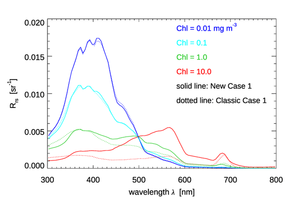
To illustrate the quantitative differences (including the combined effects of absorption and scattering coefficients and the particle scattering phase function) between the classic and new Case 1 IOP models, Fig. 8 shows the remote-sensing reflectance for homogeneous, infinitely deep waters with , as computed for the classic and new Case 1 IOP models. The mid-range UV absorption model was used in the new model. The sun was placed at a zenith angle of 30 deg in a clear sky with typical marine atmospheric parameters (sky irradiances were computed using the RADTRAN-X sky irradiance model for the annual average Earth-Sun distance). The wind speed was . For the classic IOP model, the particle phase function was taken to be a Fournier-Forand phase function with a backscatter fraction as given by the empirical formula
of Ulloa et al. (1994) for at 550 nm in Case 1 waters. These IOPs were then used in the HydroLight radiative transfer model, which was run from 300 to 800 nm with 5 nm bands.
Figure 8 shows that the computed spectra are very similar for Chl = 0.01 and 0.1, but that the differences can become very large at high chlorophyll values. The maximum difference computed as 100(new - old)/old is less than 5% for Chl = 0.01 or 0.1. For , the maximum difference is less than 50% at visible wavelengths (62% at 798 nm). For , the differences are as large as 254% (more than a factor of three; at 578 nm). The larger for high Chl is due to the greatly increased scattering, as seen in Fig. 7.
 See comments posted for this page and leave your own.