Aerosols

Aerosol Properties

Aerosols are solid or liquid particles that are much larger than gas molecules but small enough to remain suspended in the atmosphere for periods of hours to days or longer. Typical sizes are 0.1 to $10\mu m$. An aerosol’s optical properties are determined by its composition, usually parameterized via its complex index of refraction, and its particle size distribution (PSD).

For the purposes of atmospheric correction, aerosol particle size distributions are modeled as a sum of “fine” (small; radii less than roughly $1\mu m$) and “coarse” (large; radii greater than roughly $1\mu m$) particles, with a log-normal distribution for each. (The log-normal distribution is discussed on the Particle Size Distributions page and is reviewed in Campbell (1995). That page also discusses the relations between particle number, area, and volume size distributions.) The cumulative volume distribution is then (Ahmad et al. (2010))

$$\frac{dV\left(r\right)}{dlnr}=\sum _{i=1}^2\frac{V_{oi}}{\sqrt{2\pi }{\sigma }_i}exp\left[-{\left(\frac{lnr-ln{r}_{voi}}{\sqrt{2}{\sigma }_i}\right)}^2\right].$$

Here $V\left(r\right)$ is the volume of particles per volume of space with size less than or equal to $r$; $V\left(r\right)$ is typically specified as $\mu m^{3}c{m}^{-3}$. $r_{voi}$ is the volume geometric mean radius, and ${\sigma }_i$ is geometric standard deviation for class $i$. The integral of $dV\left(r\right)∕dlnr$ over all sizes $r=0$ to $\infty$ (i.e., $lnr$ from $-\infty$ to $\infty$) gives $V\left(\infty \right)=V_{oi}$. Thus $V_{oi}$ is the total volume of particles of class $i$ per volume of space.

A similar equation holds for the cumulative number distribution $dN\left(r\right)∕dlnr$, where $N\left(r\right)$ is the number of particles per volume of space with size less than or equal to $r$. The corresponding parameters $r_{noi}$ and $N_{oi}$ can be obtained from $r_{voi}$ and $V_{oi}$; see the equations in Ahmad et al. (2010). The particle size distribution (PSD) is given by

$$n\left(r\right)=\frac{dN\left(r\right)}{dr}=\frac{1}{r}\frac{dN\left(r\right)}{dlnr},$$

where $n\left(r\right)dr$ is the number of particles per unit volume in size range $r$ to $r+dr$. The units for $n\left(r\right)$ are usually expressed as $particles{m}^{-3}\mu m^{-1}$.

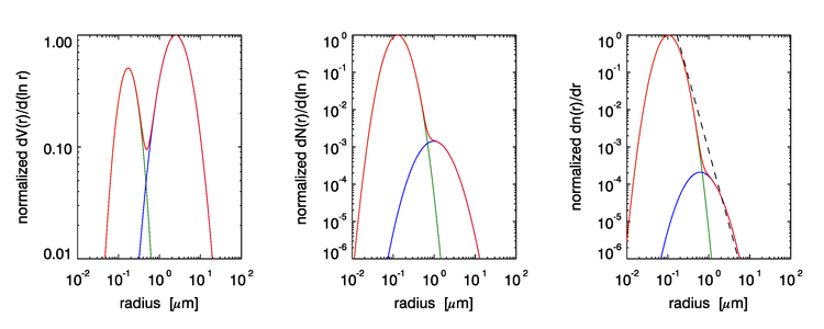
Figure 1 illustrates shapes of the volume $V\left(r\right)$, number $N\left(r\right)$, and particle size $n\left(r\right)$ distributions for an open ocean aerosol, computed using the parameter values of Table 2 of Ahmad et al. (2010). The distributions of the fine aerosols are given by the green lines. The blue lines are the coarse aerosols, and the red lines are the sums. The two roughly comparable distributions of left panel of the figure show that the fine and coarse aerosols each contribute a significant amount of the total particle volume. In the present example the fines are 25.7% of the total volume and the coarse particles are 74.3% of the total volume. The middle panel shows that the fines dominate the number of particles; in the present case there are 477 times as many fine particles as coarse. The right panel shows the PSD. The black dashed line shows the -4 slope of a Junge distribution for comparison.

---

---

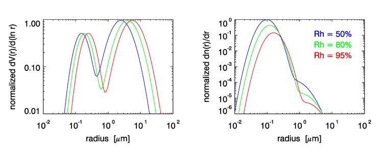
The radius parameter $r_{voi}$ and index of refraction both depend on the aerosol type (dust, sea salt, soot, etc.) and on the relative humidity $Rh$. The index of refraction generally depends on wavelength. Figure 2 shows the effect of relative humidity on cumulative volume and particle size distributions for an open-ocean aerosol (parameter values from Table 4 of Ahmad et al. (2010)). Note that as $Rh$ increases, the particles absorb more water and increase in size, so the distributions shift to the right. The shape of the distribution also changes with $Rh$.

---

---

As modeled in Ahmad et al. (2010), the fine particles are generally of ”continental” origin and include both dust and soot. The fine particles are sometimes absorbing. The coarse particles are of ”oceanic” origin and are assumed to be non-absorbing sea salts. The tables in Ahmad et al. (2010) give the PSD parameters and indices of refraction for different aerosol types (dust, sea salt, soot, etc.) and relative humidities. (Note that Table 1 of Ahmad et al. (2010) has errors. The corrected table is given in Ahmad et al. (2010b).)

An aerosol’s physical properties determine its optical properties, namely its mass-, number-, or volume-specific absorption $a^{\ast }\left(\lambda \right)$ and scattering $b^{\ast }\left(\lambda \right)$ coefficients and scattering phase function $\tilde{\beta }\left(\psi ,\lambda \right)$, where $\psi$ is the scattering angle. If the particles are homogeneous spheres, Mie theory can be used to compute the optical properties from the physical properties. This is often done, although the assumption of homogeneous spherical particles may or may not be valid in a given situation. In any case, once the $a^{\ast }\left(\lambda \right)$ and scattering $b^{\ast }\left(\lambda \right)$ coefficients are known, then given the concentration profile $Conc\left(z\right)$ as a function of altitude $z$, the extinction coefficient $c\left(z,\lambda \right)=Conc\left(z\right)\left[a^{\ast }\left(\lambda \right)+b^{\ast }\left(\lambda \right)\right]$ can be computed. The aerosol optical thickness or aerosol optical depth is then given by

$${\tau }_a\left(\lambda \right)={\int \; <!--nolimits-->}_{z_0}^{TOA}c\left(z,\lambda \right)dz,$$

where $z_0$ is the surface elevation. (Generally $z_0=0$ for mean sea level, but may also be the elevation of a lake.)

For all else held fixed, the aerosol optical thickness at wavelength $\lambda$ is approximately related to the value at a reference wavelength ${\lambda }_o$ by

$$\frac{{\tau }_a\left(\lambda \right)}{{\tau }_a\left({\lambda }_o\right)}={\left(\frac{{\lambda }_o}{\lambda }\right)}^{\alpha }$$

(1)

The parameter $\alpha$ is known as the Ångström exponent or Ångström coefficient. Smaller (larger) particles generally have a larger (smaller) Ångström exponent.

The single scattering albedo ${\omega }_o$ defined by

$${\omega }_o\left(\lambda \right)=\frac{b^{\ast }\left(\lambda \right)}{c^{\ast }\left(\lambda \right)}$$

is also of use in modeling the optical effects of aerosols on the radiance distribution.

Ahmad et al. (2010) constructed look-up-tables (LUTs) for 10 aerosol types and 8 relative humidities, for a total of 80 aerosol tables. The fine fraction was a mixture of 99.5% dustlike and 0.5% soot particles (not modeled by Shettle and Fenn) for all 10 aerosol types, which gives good agreement on average with AERONET measurements of aerosol optical properties. The ten aerosol models have different weights of fine and coarse particles, but the effective radius $r_{eff}$ ($r_{eff}=\int \; <!--nolimits-->r^{3}n\left(r\right)dr∕\int <!--nolimits-->r^{2}n\left(r\right)dr$) and mean radius ${\mu }_o$ (${\mu }_o=\int \; <!--nolimits-->rn\left(r\right)dr∕\int \; <!--nolimits-->n\left(r\right)dr$) are the same. The aerosol types were then defined by letting the fine-to-coarse fraction vary from 0 to 1. For each aerosol type, relative humidities of $Rh$ = 30, 50, 70, 75, 80, 85, 90, and 95% were used. The actual aerosol LUTs contain the components of the model from which to derive single-scattering aerosol reflectance ratios in each band (relative to any reference band), plus a set of quadratic coefficients relating single to multiple scattering (as in Gordon and Wang (1994a)), plus a separate table of Rayleigh-aerosol diffuse transmittance coefficients of the form $t=Aexp\left(-B{\tau }_a\right)$ (recall Eq. (6) of the Atmospheric Transmittances page). Mie is theory used to compute the aerosol phase functions for use in the radiative transfer model.

Black-pixel Calculations

The algorithm developed by Gordon and Wang (1994a) is used, although the original aerosol models and LUTs have been updated as described in Ahmad et al. (2010), and model selection is now partitioned by relative humidity ($Rh$). (Gordon and Wang ignored the glint term since they were considering SeaWiFS, whose viewing direction was chosen to avoid direct Sun glint.)

Beginning with Eq. (13) of the Normalized Reflectances page,

$${\rho }_t={\rho }_R+\left[{\rho }_a+{\rho }_{Ra}\right]+T{\rho }_g+t{\rho }_{wc}+t{\rho }_w,$$

(2)

The basic theory in Gordon and Wang (1994a) is developed using single-scattering theory, in which case the ${\rho }_{Ra}$ term is zero because there is no multiple scattering. Multiple-scattering effects are then added via numerical models using the guidance of the single-scattering theory.

Assume that the corrections for Rayleigh, whitecaps, $O_3$, ${NO}_2$, and Sun glint have all been made. Then the left hand side of

$${\rho }_t-{\rho }_R-T{\rho }_g-t{\rho }_{wc}=\left[{\rho }_a+{\rho }_{Ra}\right]+t{\rho }_w$$

(3)

or

$${\rho }_{Aw}\equiv {\rho }_A+t{\rho }_w$$

is known. Here ${\rho }_{Aw}$ is just convenient shorthand for the measured TOA reflectance ${\rho }_t$ with the Rayleigh and other effects removed. The next task is to compute ${\rho }_A$, the combined aerosol and aerosol-Rayleigh reflectance, and move it to the left hand side, after which the desired ${\rho }_w$ will be known.

Low-chlorophyll, Case 1 waters have negligible water-leaving radiance at near-infrared (NIR) wavelengths, i.e. beyond roughly 700 nm. For such waters, it can be assumed that ${\rho }_w\left(\lambda >700nm\right)=0$, which is known as the ”black-pixel” assumption. Let ${\lambda }_1$ and ${\lambda }_2$ be two NIR wavelengths, with ${\lambda }_1<{\lambda }_2$. At these two wavelengths, the TOA normalized reflectance (corrected as shown in Eq. (3)) is due entirely to atmospheric path radiance: ${\rho }_{Aw}\left({\lambda }_i\right)={\rho }_A\left({\lambda }_i\right),i=1,2$. Table 1 shows the ${\lambda }_1$ and ${\lambda }_2$ bands for several sensors.

Now consider the ratio

$$𝜖\left({\lambda }_1,{\lambda }_2\right)\equiv \frac{{\rho }_A\left({\lambda }_1\right)}{{\rho }_A\left({\lambda }_2\right)}\underset{\text{Black Pixel}}{=}\frac{{\rho }_{Aw}\left({\lambda }_1\right)}{{\rho }_{Aw}\left({\lambda }_2\right)}$$

(4)

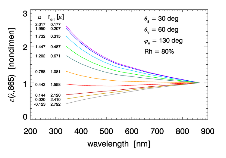
The quantity $𝜖\left({\lambda }_1,{\lambda }_2\right)$, and more generally the quantity $𝜖\left(\lambda ,{\lambda }_2\right)$ for any $\lambda <{\lambda }_2$, depends on the aerosol type, which is determined by the particle type, PSD, and relative humidity. Figure 3 shows the dependence of $𝜖\left(\lambda ,{\lambda }_2=865\right)$ for the ten aerosol models, for one particular set of solar zenith angle, viewing direction, and relative humidity.

---

---

For the given image pixel being corrected, the process is as follows:

• The relative humidity $Rh$ is taken from NCEP.
• For each bounding $Rh$ value in the family of 8 $Rh$ values in the database, the corresponding family of 10 aerosol types in the database is then searched to find the two aerosols types whose precomputed values of $𝜖\left({\lambda }_1,{\lambda }_2\right)$, call them ${𝜖}_{low}$ and ${𝜖}_{high}$, bracket the measured value of $𝜖\left({\lambda }_1,{\lambda }_2\right)$ for the given Sun and viewing geometry.
• This selects two of the curves like those of Fig. 3, for which the corresponding $𝜖\left(\lambda ,{\lambda }_2\right)$ and ${\tau }_a$ values have been precomputed and stored in the aerosol LUT.
• It is assumed that the difference in the precomputed $𝜖\left(\lambda ,{\lambda }_2\right)$ is at all wavelengths in the same proportion as the measured $𝜖\left({\lambda }_1,{\lambda }_2\right)$ is to the bracketing values at the NIR reference wavelengths. Thus let

  $$\Delta =\frac{𝜖\left({\lambda }_1,{\lambda }_2\right)-{𝜖}_{low}\left({\lambda }_1,{\lambda }_2\right)}{{𝜖}_{high}\left({\lambda }_1,{\lambda }_2\right)-{𝜖}_{low}\left({\lambda }_1,{\lambda }_2\right)}$$

  (5)

• The aerosol reflectance at all wavelengths is then computed from the measured ${\rho }_{Aw}\left({\lambda }_2\right)$ and the tabulated ${𝜖}_{low}$ and ${𝜖}_{high}$ values using

  $${\rho }_A\left(\lambda \right)=\left[\left(1-\Delta \right){𝜖}_{low}\left(\lambda ,{\lambda }_2\right)+\Delta {𝜖}_{high}\left(\lambda ,{\lambda }_2\right)\right]{\rho }_{Aw}\left({\lambda }_2\right)$$

  (6)

Now that ${\rho }_A\left(\lambda \right)$ is known, Eq. (3) gives

$$t{\rho }_w={\rho }_{Aw}-{\rho }_A={\rho }_t-{\rho }_R-T{\rho }_g-t{\rho }_{wc}-\left[{\rho }_a+{\rho }_{Ra}\right]$$

(7)

Recall that $t$ is the diffuse transmission in the viewing direction, and that $t{\rho }_w$ is the contribution of water-leaving radiance (in reflectance form) at the TOA. The desired ${\rho }_w$ at the sea surface is thus obtained from

$${\rho }_w=\frac{{\rho }_{Aw}-{\rho }_A}{t}.$$

(8)

The aerosol optical depth is computed at all wavelengths using the values of $\tau \left({\lambda }_2\right)$ and the Ångström exponent in Eq. (1).

This technique rests on two main assumptions:

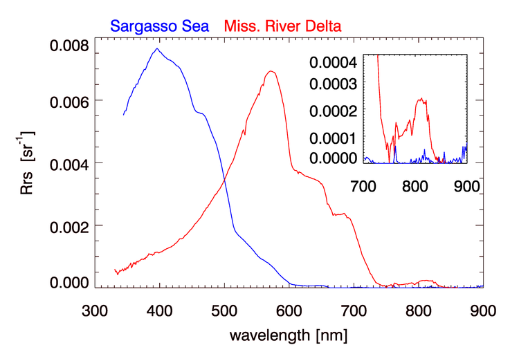
• The water-leaving radiance is negligible at the NIR reference wavelengths. This is valid only for optically deep, Case 1 waters, with a chlorophyll concentration of $0.3mg{m}^{-3}$ or less. Waters containing higher chlorophyll concentrations or mineral particles will violate this assumption. Figure 4 shows an example of very turbid water for which the remote-sensing reflectances at NIR wavelengths is not negligible.
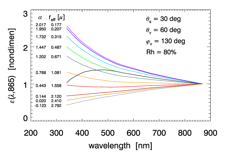
• The aerosols are not strongly absorbing. Some mineral aerosols absorb strongly at blue wavelengths but not in the NIR. Their $𝜖\left(\lambda ,{\lambda }_2\right)$ functions look like the black curve in Fig. 5. Thus their presence cannot be detected from the NIR TOA radiances.

Note that these are unrelated assumptions: the water can have non-zero NIR reflectance and the atmosphere can have non-absorbing aerosols, or there can be zero NIR reflecance but absorbing aerosols. If the water-leaving radiance is not zero at the ${\lambda }_2$ reference wavelength, then the ${\rho }_w$ contribution to ${\rho }_{Aw}$ will be interpreted as a larger aerosol concentration. This leads to over-correction for the aerosol, i.e, subtracting too much ${\rho }_A$ from ${\rho }_{TOA}$. The resulting ${\rho }_w$ is then too small, and can even be negative at blue wavelengths. Likewise, if the aerosol is blue-absorbing, over-correction occurs at blue wavelengths and, again, ${\rho }_w$ is too small or even negative at blue wavelengths.

---

---

---

---

Non-black-pixel Calculations

Many ways to treat non-black pixels have been developed; the method currently implemented by the OBPG is described in Bailey et al. (2010). This algorithm works as follows.

It is necessary to estimate $R_{rs}\left(\lambda \right)$ (or equivalently ${\rho }_w\left(\lambda \right)$) at the NIR reference wavelengths so that the non-zero water-leaving radiance can be removed from the TOA signal, leaving only the aerosol reflectance as the contribution to ${\rho }_{Aw}$, from which the aerosol type (i.e., $𝜖\left(\lambda ,{\lambda }_2\right)$) can be determined. However, $R_{rs}\left(NIR\right)$ can’t be estimated until the aerosol contribution is removed. Thus an iterative solution must be used to obtain both $R_{rs}\left(NIR\right)$ and the aerosol type.

The remote-sensing reflectance can be written

$$R_{rs}\left(\lambda \right)=\frac{f\left(\lambda \right)}{Q\left(\lambda \right)}\frac{b_b\left(\lambda \right)}{a\left(\lambda \right)+b_b\left(\lambda \right)}.$$

(9)

As discussed in detail on the Normalized Reflectances page, the $f∕Q$ factor describes the angular distribution of the water-leaving radiance, i.e., the BRDF of the ocean. This factor depends on the Sun and sky radiance distribution (parameterized by the solar zenith angle ${𝜃}_s$ and AOT ${\tau }_a$), water-column IOPs (parameterized by the chlorophyll concentration $Chl$ in Case 1 waters), sea state (wind speed $W$), viewing direction (${𝜃}_v,{\varphi }_v$), and wavelength. It has been extensively studied and numerically modeled by Morel et al. (2002), who present tabulated values as functions of ${𝜃}_s,{\tau }_a,{𝜃}_v,{\varphi }_v,Chl,W$, and $\lambda$. Although the Morel et al. (2002) $f∕Q$ table was generated for Case 1 waters, analysis shows (Bailey et al. (2010)) that it is often adequate for Case 2 waters as well. The $f∕Q$ factor is thus considered known for the present calculations.

The iterative correction for waters where the black-pixel assumption cannot be made has the following steps:

1.

Assume that $R_{rs}\left(765\right)$ and $R_{rs}\left(865\right)$ are both 0, i.e. make the black-pixel assumption for both NIR reference bands.

2.

Complete the atmospheric correction process as described for black pixels. This gives the initial estimate of ${\rho }_w\left(\lambda \right)$, or equivalently $R_{rs}\left(\lambda \right)$.

3.

Use $R_{rs}\left(443\right)$ and $R_{rs}\left(555\right)$ from the initial estimate of $R_{rs}\left(\lambda \right)$ to get $\eta$ by the empirical relationship (Lee et al. (2010b), Eq. 8; Bailey et al. (2010), Eq. 3)

$$\eta =2\left[1-1.2exp\left(0.9\frac{R_{rs}\left(443\right)}{R_{rs}\left(555\right)}\right)\right].$$

(10)

4.

Use the initial $R_{rs}\left(\lambda \right)$ to get an initial estimate of the chlorophyll concentration $Chl$. The particular algorithm used to obtain $Chl$ from $R_{rs}\left(\lambda \right)$ depends on the sensor.

5.

Use this $Chl$ to obtain $a\left(670\right)$ via the empirical relationship (Bailey et al. (2010), Eq. 4)

$$a\left(670\right)=exp\left[0.9389ln\left(Chl\right)-3.7589\right]+a_w\left(670\right).$$

(11)

where the $a_w\left(670\right)=0.439m^{-1}$ is the absorption by pure water.

6.

Use $a\left(670\right)$ and $R_{rs}\left(670\right)$ in Eq. (9) to solve for $b_b\left(670\right)=b_{bw}\left(670\right)+b_{bp}\left(670\right)$, where $b_{bw}\left(670\right)=4.26\times 10^{-4}{m}^{-1}$ is the backscatter coefficient for pure sea water.

7.

Use $\eta$ from Eq. (10) and Bailey et al. (2010), Eqs. (2b) and (3) to compute $b_b\left(765\right)$:

$$b_b\left(765\right)=b_{bw}\left(765\right)+b_{pb}\left(670\right){\left(\frac{670}{765}\right)}^{\eta }$$

(12)

where $b_{bw}\left(765\right)=2.38\times 10^{-4}{m}^{-1}$. $b_b\left(865\right)$ is computed in the same manner using $b_{bw}\left(865\right)=1.41\times 10^{-4}{m}^{-1}$.

8.

Use this $b_b\left(765\right)$ and $a\left(765\right)=a_w\left(765\right)=2.85m^{-1}$ to get $R_{rs}\left(765\right)$ from Eq. (9). Similarly, compute $R_{rs}\left(865\right)$ using $b_b\left(865\right)$ and $a_w\left(865\right)=4.61m^{-1}$.

9.

Use the new, non-zero value of $R_{rs}\left(765\right)$ (i.e. ${\rho }_w\left(765\right)$) to remove the non-zero ${\rho }_w\left(765\right)$ contribution to ${\rho }_t\left(765\right)$. Do the same calculation for 865 nm.

10.

Return to Step 2 and repeat the atmospheric correction using the black-pixel algorithm. This will give a new (hopefully better) estimate of $R_{rs}\left(\lambda \right)$, thus an new estimate of the other parameters, and finally new estimates of $R_{rs}\left(765\right)$ and $R_{rs}\left(865\right)$ at Step 8. After using the new values of ${\rho }_w\left(765\right)$ and ${\rho }_w\left(865\right)$ to correct for the non-zero water contribution to ${\rho }_t\left(765\right)$ and ${\rho }_t\left(865\right)$, return to Step 2 for a new iteration. Continue iterating until the change in $R_{rs}\left(765\right)$ from one iteration to the next is less than 2%, which typically takes 2-4 iterations, or when 10 iterations have been made.

If this iteration process fails to converge within 10 cycles, then re-initialze with ${\rho }_a\left(NIR\right)=0$, i.e., set the NIR aerosol contribution to zero. This implies that all of the NIR reflectance is due to the water (after correction for Rayleigh and Sun glint). Repeat the iteration until convergence is reached. If convergence is still not reached, do one more calculation with ${\rho }_a\left(NIR\right)=0$ and flag the pixel as ”atmospheric correction warning.” However, even in this case, the retrieval may still be useful.

The above iteration is not done if the initial $Chl$ estimate is less that $0.3mg{m}^{-3}$, and it is always done if the initial $Chl$ estimate is greater that $0.7mg{m}^{-3}$. To prevent discontinuities in the final results, the $R_{rs}\left(765\right)$ estimate is linearly weighted from 0 to 1 for $0.3\le Chl\le 0.7$. Figure 6 shows the regions of the ocean where the non-black-pixel algorithm is likely to be applied.

---

---

Finally, rather than the exact NIR reference wavelengths of ${\lambda }_1=765$ and ${\lambda }_2=865$ shown above, in practice band-averaged IOP values are used for the particular sensor. Thus for VIIRS-NPP, the reference bands are centered at 745 and 862 nm, with the band-averaged $a_w\left(745\right)=2.806m^{-1}$, and so on. Band averaged IOPs for different sensors are given at NASA ocean color documents.

Strongly Absorbing Aerosols

The aerosol models of Ahmad et al. (2010) discussed in Section include a small fraction of absorbing soot for the fine part of the aerosol size distribution. These aerosol models are used for routine correction for aerosols. These models, however, cannot account for the presence of strongly absorbing aerosols, which frequently occur in coastal regions downwind from continents, and even in mid-ocean regions because winds can transport fine dust particles long distances.

Strongly absorbing aerosols (especially at blue wavelengths) have been a topic of much research over the years, e.g., Gordon et al. (1997b). However, as was illustrated in Fig. 5, there is no reliable way to detect the presence of absorbing aerosols from the NIR bands of Table 1 during the atmospheric correction process. Therefore, all pixels are processed using the algorithms for non- or weakly absorbing aerosols as described in the previous sections.