The Asymptotic Radiance Distribution

Deep in homogeneous, source-free waters the radiance distribution $L\left(z,𝜃,\varphi \right)$ approaches a shape $L_{\infty }\left(𝜃\right)$ that depends only on the IOPs. Moreover, the radiance distribution at great depth decays in magnitude exactly exponentially with a decay rate $K_{\infty }$ that, once again, depends only on the IOPs. The shape $L_{\infty }\left(𝜃\right)$ is called the asymptotic radiance distribution, and $K_{\infty }$ is called the asymptotic decay rate or the asymptotic K function. $L_{\infty }\left(𝜃\right)$ and $K_{\infty }$ depend on the wavelength $\lambda$ via the wavelength dependence of the IOPs; the wavelength is omitted here for brevity. An asymptotic radiance distribution exists only if the IOPs do not depend on depth (homogeneous water) and if there is no inelastic scatter or bioluminescence contributing to the radiance (source-free water). Preisendorfer (1976) (in Hydrologic Optics, vol. 5, page 212) and Højerslev and Zaneveld (1977) give rigorous mathematical proofs that $L_{\infty }\left(𝜃\right)$ and $K_{\infty }$ exist for any physically realistic phase function and single-scattering albedo.

These statements imply that the directional and depth dependencies of the radiance distribution decouple at great depths. That is to say,

This in turn implies that all irradiances decay in the asymptotic regime at the same rate as the radiance. For example,

We can compute corresponding values for $E_u$, $E_{od}$, and $E_{ou}$. Clearly, each of these irradiances has the same asymptotic K function. Using these asymptotic irradiances, we can compute asymptotic values for any apparent optical property. For example, we have

Note that any normalization factor in $L_{\infty }\left(𝜃\right)$ divides out when computing AOPs.

Because the asymptotic radiance $L_{\infty }\left(𝜃\right)$ is determined solely by the IOPs, it follows that any quantity computed from $L_{\infty }\left(𝜃\right)$ is also in IOP. Therefore all apparent optical properties become inherent optical properties in the asymptotic regime. The K’s, $\overline{\mu }$’s, R’s, and their ilk, which are influenced by boundary conditions near the water surface, all approach values at depth that are independent of the boundary conditions.

An Integral Equation for the Asymptotic Radiance Distribution

The obvious question is, “How do you computed the asymptotic radiance distribution and the asymptotic decay rate, given the IOPs?” One way is to recall the RTE for homogeneous, source-free water

and assume that the radiance has the form seen in Eq. (1). This gives an integral equation for the shape $L_{\infty }\left(𝜃\right)$ and decay rate $K_{\infty }$ of the asymptotic radiance distribution:

(Note that since the scattering angle $\psi$ depends only on $cos\left(\varphi -{\varphi }^{\prime }\right)$, we can set $\varphi =0$ in this equation, so that the result is a function only of $𝜃$.) This equation is often written in terms of $\mu =cos𝜃$ and a nondimensional asymptotic decay rate ${\kappa }_{\infty }=K_{\infty }∕c$ as

Given the IOPs $c$ and $\beta$ for Eq. (2) or ${\omega }_o$ and $\tilde{\beta }$ for Eq. (3), we can solve either of these equations for the corresponding $L_{\infty }$ and $K_{\infty }$ or ${\kappa }_{\infty }$. Another form of Eq. (3), often seen in the literature, is

where $h\left({\mu }^{\prime },\mu \right)$ is the azimuthally averaged phase function

For the idealized case of isotropic scattering, $\tilde{\beta }=1∕4\pi$ and the solution of Eq. (3) has the simple form

where $L_{\infty }\left(\mu \right)$ is normalized to 1 at $\mu =1$ (or at the nadir direction $𝜃=0$). This $L_{\infty }\left(\mu \right)$ has the shape of an ellipse whose major axis is oriented vertically. The corresponding value of ${\kappa }_{\infty }$ is the solution of the transcendental equation

as can be seen by substitution of Eq. (4) into Eq. (3).

Kattawar and Plass (1976) obtained an analytic solution of Eq. (3) for the Rayleigh phase function $\tilde{\beta }=\left(3∕16\pi \right)\left(1+{cos}^2\psi \right)$. However, for other phase functions, in particular for those characteristic of oceanic waters, the solution of Eq. (2) or (3) must be obtained numerically.

Solving the integral Eq. (2) is mathematically equivalent to solving a certain eigenmatrix equation for its eigenfunctions (which give $L_{\infty }$) and eigenvalues (which give $K_{\infty }$). The eigenmatrix approach is described in Light and Water (1994) section 9.6. (HydroLight uses the eigenmatrix approach to obtain its asymptotic values. The excellent agreement between the asymptotic values computed by the eigenmatrix method and the approach with depth to those values, as obtained by independent numerical solution of the RTE, is an excellent check on the correctness of the HydroLight code.)

Dependence of Asymptotic Values on Inherent Optical Properties

As just seen, the two asymptotic properties $L_{\infty }$ and $K_{\infty }$ are determined solely by the IOPs $c$, ${\omega }_o$ and $\tilde{\beta }$. Figure 1 shows how the nondimensional asymptotic decay rate ${\kappa }_{\infty }=K_{\infty }∕c$ depends on the albedo of single scattering ${\omega }_o$ for three phase functions. The dotted line is for the pure water phase function ${\tilde{\beta }}_w$; the dashed line is for a Henyey-Greenstein phase function ${\tilde{\beta }}_{HG}$ with an asymmetry parameter $g=0.7$; and the solid line is for a Petzold “average-particle” phase function ${\tilde{\beta }}_p$, which is typical of phase functions for oceanic particles. The squares show experimental data taken in laboratory suspensions containing milk (Timofeeva and Gorobetz, 1967). The fat globules in milk are large ($\gg \lambda$), efficient scatterers, which explains the similarity between the milk solution and the ${\tilde{\beta }}_p$ phase function, which is typical of particle-laden natural waters.

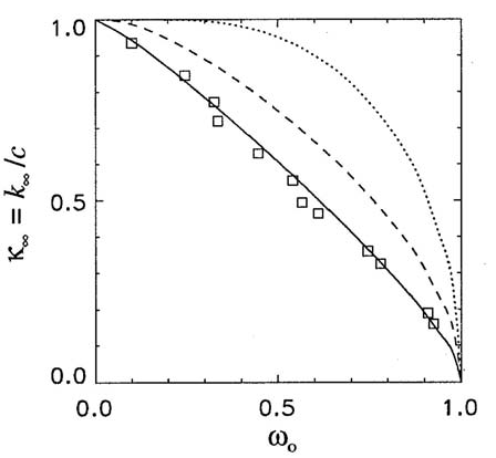
Figure 2 shows the shape of $L_{\infty }\left(𝜃\right)$ as a function of ${\omega }_o$ for the average-particle phase function ${\tilde{\beta }}_p$. Since it is the shape that is determined by the IOPs, it is customary to normalize $L_{\infty }\left(𝜃\right)$ to one for the nadir radiance direction (looking upward in the zenith direction). The viewing angle ${𝜃}_v$ as plotted is the angle in which an underwater observer would look in order to see radiance traveling in direction $𝜃=180^{\circ }-{𝜃}_v$; ${𝜃}_v$ and $𝜃$ are both measured from the $+ẑ$, or nadir, direction. Thus, ${𝜃}_v=180^{\circ }$ corresponds to looking toward the zenith and seeing radiance heading straight down ($𝜃=0$). As we would expect, in highly scattering water (large ${\omega }_o$) the upwelling radiance is relatively much greater than in weakly scattering water (small ${\omega }_o$). Corresponding curves for the Rayleigh phase function can be seen in Kattawar and Plass (1976). Prieur and Morel (1971) show such curves as a function of the relative contributions by molecular and particle scattering, i.e., for phase functions that are in between ${\tilde{\beta }}_w$ and ${\tilde{\beta }}_p$.

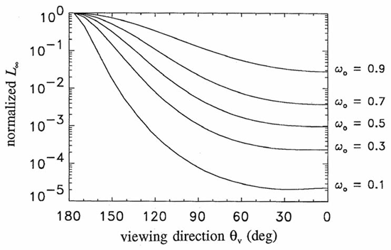
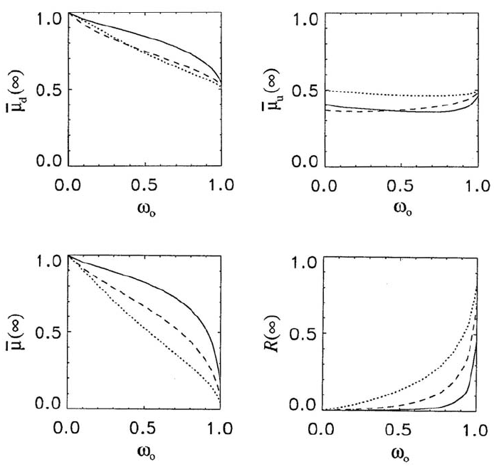
Figure 3 shows the asymptotic mean cosines and irradiance reflectance for the same phase functions used in Fig. 1.

Rate of Approach to Asymptotic Values

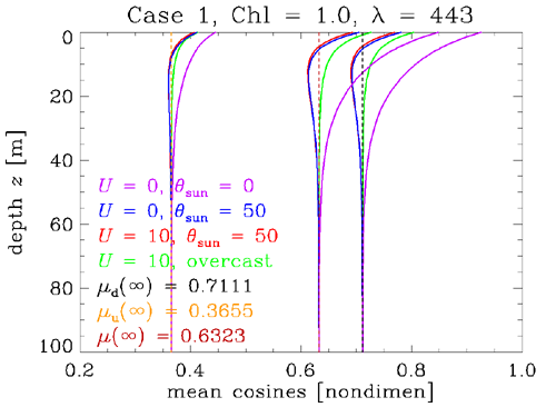
The asymptotic values are determined solely by the IOPs of a homogeneous water body. However, how quickly a given quantity approaches its asymptotic value depends on both the IOPs and the boundary conditions. We have already seen this in the discussion of K functions, but a few more examples will be instructive. HydroLight was run for Case 1 water with a chlorophyll concentration of $Chl=1.0mg{m}^{-3}$. The wavelength was 443 nm. The corresponding IOPs (including water) were $a=0.0680m^{-1}$, $b=0.4346m^{-1}$, so that $c=0.5026m^{-1}$. Thus one meter of geometric depth is about 0.5 optical depths. The albedo of single scattering is then ${\omega }_o=b∕c=0.8648$, and the total backscatter fraction was 0.1253. Figure 4 shows $K_d$ at 443 nm for four different surface boundary conditions:

• the Sun is at the zenith in a clear sky (${𝜃}_{sun}=0$) and the sea surface is level (wind speed $U=0$)
• the Sun is at a 50 deg zenith angle in a clear sky (${𝜃}_{sun}=50$) and the sea surface is level ($U=0$)
• the Sun is at a 50 deg zenith angle in a clear sky (${𝜃}_{sun}=50$) and the sea surface is wind blown, with a wind speed of 10 m/s ($U=10$)
• the sky has a cardioidal radiance distribution, $L\left(𝜃,\varphi \right)=L_o\left(1+2cos𝜃\right)$, $0\le 𝜃\le \pi ∕2$, which is similar to a heavy overcast through which the location of the Sun cannot be determined, and the sea surface is wind blown, with a wind speed of 10 m/s ($U=10$)

The curves of Fig. 4 show the boundary effects on the rate of approach to the asymptotic value of $K_{\infty }=0.1075m^{-1}$, which depends only on the IOPs. The curve for the heavily overcast sky approaches $K_{\infty }$ the quickest. The physical reason is that the overcast sky radiance is already a diffuse radiance distribution, so that less scattering (i.e., less propagation to depth) is required to redirect the initial photon directions towards the asymptotic angular distribution within the water. The other cases with the sun in a clear sky have a strongly collimated incident radiance distribution, which requires more scattering (a deeper depth) to “erase the memory” of where the sun is in the sky and achieve the asymptotic shape of $L_{\infty }\left(𝜃\right)$ . For the 50 deg Sun zenith angle, the surface roughness makes a noticeable but minor difference.

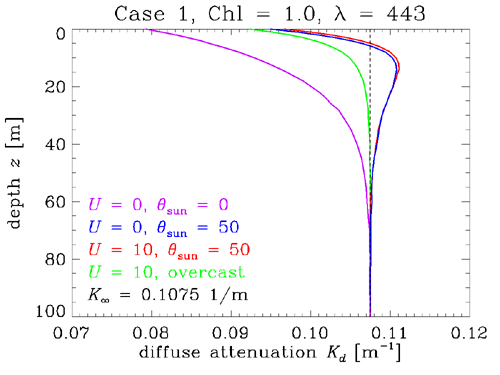
Figure 5 shows the corresponding results for the approach of the irradiance reflectance $R=E_u∕E_d$ to its asymptotic value of $R_{\infty }=0.0406$.

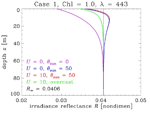
Fig. 6 shows the mean cosines ${\overline{\mu }}_d$, ${\overline{\mu }}_u$, and $\overline{\mu }$.

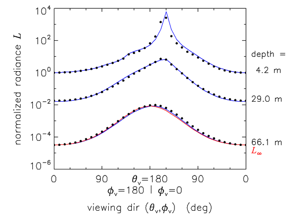
Finally, Fig. 7 shows the approach of measured and modeled radiances to the asymptotic shape. The dots are radiances measured in the azimuthal plane of the Sun by Tyler (1960) at the depths indicated. The blue curves are the corresponding HydroLight simulation. The measured data were published only as relative values. Therefore, the radiances are normalized for plotting to a value of 1 in the nadir-viewing direction (${𝜃}_v=0$) at depth 4.2 m. The ${\varphi }_v=0$ direction is looking toward the sun, and ${\varphi }_v=180$ is looking away from the sun. The red curve shows the shape of $L_{\infty }$, normalized to the nadir-viewing measured value at 66.1 m. The data are described in detail in Tyler’s report, and the modeling is described in Light and Water (1994) section 11.1. Given the uncertainties in the measured data and the educated guesses that had to be made about unmeasured inputs needed by HydroLight, the overall agreement between data and model predictions is quite good.

Near the surface, the Sun’s location is obvious and the unscattered direct beam gives a large spike in the radiance. At 29.0 m, the sun’s azimuthal direction can still be discerned, but the large spike of the direct beam has been removed by scattering. By 66.1 m, there is only a slight asymmetry remaining to indicate the sun’s azimuthal direction. Clearly, both the measured and modeled radiances are close to the asymptotic shape at 66.1 m, which was about 26 optical depths.