Visualizing VSFs

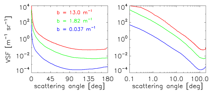
Oceanic volume scattering functions typically vary by 5 or 6 orders of magnitude over the range of very small to large scattering angles. Figure 1 illustrates the range of VSFs than can be found in various oceanic waters. Each of these VSFs varies by over ﬁve orders of magnitude between a scattering angle of $ψ$ = 0.1 deg and their minima at large angles. The diﬀerent VSFs vary by over two orders of magnitude at a given scattering angle.

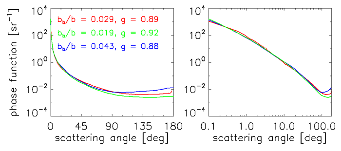
Figure 1: Example volume scattering functions. The blue curve was measured in clear, open ocean water; the wavelength was 514 nm. The green curve was measured in a harbor (514 nm), and the red curve in very productive coastal waters (530 nm). The corresponding scattering coeﬃcients b are shown in the left panel.

The phase functions computed from these three VSFs are plotted in Fig. 2. The left panel shows the backscatter fractions and asymmetry parameters for each phase function. Although these phase functions appear similar in shape, at least when plotted with a logarithmic ordinate, there are signiﬁcant diﬀerences. Note in particular that they vary by almost an order of magnitude at large scattering angles, and their backscatter fractions vary by over a factor of two. Thus the diﬀerent shapes of these phase functions would give factor-of-two or greater diﬀerences in upwelling radiances as measured by remote-sensing instruments. The actual diﬀerences in upwelling radiances would be even larger because of the magnitude diﬀerences in the VSFs.

Figure 2: Example scattering phase functions. The color coding is the same as for Fig. 1

VSFs and phase functions are usually plotted as functions of the scattering angle $ψ$ , as seen in the preceding ﬁgures. The ordinate is almost always logarithmic because of the wide ranges of VSF and phase function magnitudes. The abscissa can be linear (as in the left panels) or logarithmic (right panels); a logarithmic abscissa highlights the smallest scattering angles. However, it should be remembered that scattering is an inherently three-dimensional process involving both polar and azimuthal scattering angles relative to the direction of the unscattered light.

Another typical oceanic phase function is displayed in four diﬀerent ways in Fig. 3, which is worthy of some discussion. This particular phase function has an asymmetry parameter or average cosine of $g$ = 0.897, and a backscatter fraction of $B_{b}$ = 0.0289. In the upper two plots, the magnitude of the phase function has been color coded for comparison with the three-dimensional displays seen in the lower panels of the ﬁgure.

Figure 3: A typical oceanic phase function viewed in various ways. The magnitude is color coded the same in all plots.

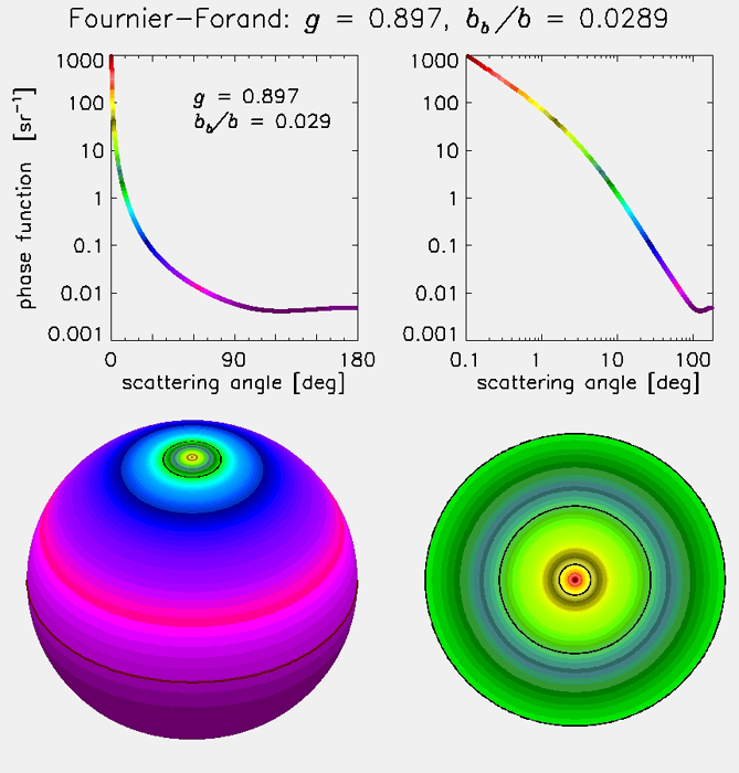
The lower-left panel gives a 3-D perspective of the phase function, with the ”north pole” of the sphere being the direction of the unscattered light. This point is colored dark red to indicate the large magnitude of the phase function, corresponding to the color scheme of the line drawings. The polar angle or ”latitude” of the sphere is the scattering angle, and the ”longitude” is the azimuthal angle of the scattering. Because we have assumed that the scattering is independent of the azimuthal angle, there is no azimuthal dependence in this 3-D plot. The black circle in the green region near the pole is $ψ$ = 10 deg. scattering angle; the dark red circle at the ”equator” is $ψ$ = 90 deg. The dark purple color in the backscatter directions at the bottom of the sphere indicates the low magnitudes of the phase function as seen in the line plots.

The lower-right plot is an expanded view of the scattering angles from 0 to 10 deg, as contained within the black circle of the lower-left sphere plot. The view is looking ”into the beam,” or toward the light source. The inner black circle is $ψ$ = 1 deg., the next black circle is $ψ$ = 5 deg., and the outer black circle is the $ψ$ = 10 deg. value seen in the sphere plot.

These four plots displace the same information in diﬀerent ways. The two plots on the left are linear in the scattering angle, and the two plots on the right emphasize the small-angle scattering. The top two plots are the usual way of showing VSFs or phase functions when the scattering is azimuthally symmetric; the bottom two plots illustrate the 3-D character of the scattering process.

Figure 4 shows the phase function for pure water, which is given by the simple formula

{\tilde{β}}_{w} (ψ) = 0.06225 (1 + 0.835 {cos}^{2} ψ) .

(1)

The pure water phase function has only a small range of magnitudes and is symmetric about the $ψ$ = 90 deg scattering angle. Therefore the asymmetry parameter or average cosine of this phase function is $g$ = 0, and the backscatter fraction is $B_{b}$ = 0.5.

Figure 4: The phase function for pure water.

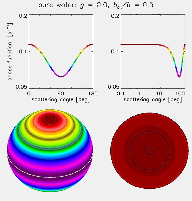
In the discussion of IOPs on the previous page, we assumed that the medium, i.e. the water, was isotropic. Note that an isotropic medium does not have isotropic scattering, which would be a VSF that is independent of the scattering angle. Isotropic scattering is an idealization that does not exist in nature. Scattering by pure water is the closest you can come to isotropic scattering in the ocean.

Visualizing VSFs

Comments for Visualizing VSFs: