Out-of-Band Response

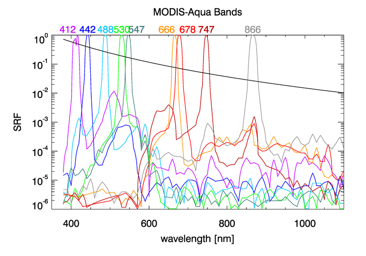
Figure 1 shows the sensor response functions (SRF) of the MODIS-Aqua bands used for ocean color remote sensing; each response function is normalized to 1 at its maximum. Visually, in this plot with a linear ordinate axis, the bands appear to be well defined and narrow, with full-width, half-maximum (FWHM; the wavelengths at which the function is one-half of its maximum) widths of 10 to 15 nm. However, when plotted with a logarithmic ordinate as in Fig. 2, it is seen that there is significant “out-of-band” (OOB) sensitivity; i.e., a non-zero response outside the nominal band width. In each plot, the black curve represents a TOA radiance with a wavelength dependence of ${\lambda }^{-4}$.

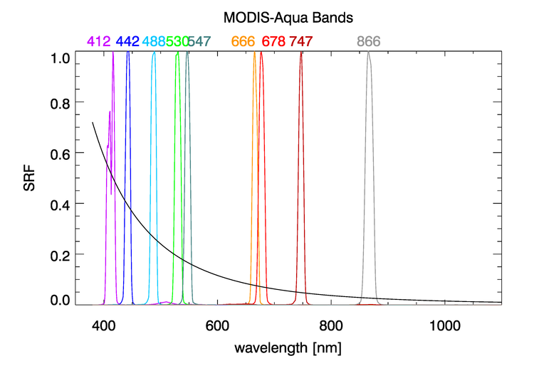
Rayleigh scattering with a ${\lambda }^{-4}$ dependence dominates the total TOA radiance. If a radiance with such a wavelength dependence is measured by sensors having the response functions shown in Figs. 1 and 2, the total measured radiance in the $i^{th}$ band over the 380-1100 nm range shown in the figures will be (Gordon (1995), Eq. 8)

Define the “in-band” part of the total signal to be the part detected between chosen lower (${\lambda }_{low}$) and upper (${\lambda }_{up}$) wavelengths. The NASA Ocean Biology Processing Group (OBPG) uses the wavelengths at which the SRF drops to 0.1% of its maximum value to define the lower and upper boundaries of the in-band region. For the nominal 488 nm band, for example, ${\lambda }_{low}=460nm$ and ${\lambda }_{up}=503nm$. (The FWHM boundaries for the 488 nm band are $FWH{M}_{low}=482nm$ and $FWH{M}_{up}=493nm$.) The part of the measured radiance that comes from in-band wavelengths is then

with similar equations for the out-of-band contributions at wavelengths less than ${\lambda }_{low}$ and greater than ${\lambda }_{up}$. Numerical integration shows that for a ${\lambda }^{-4}$ TOA radiance and the nominal 488 nm band, 99.24% comes from the in-band wavelengths, 0.55% comes from out-of-band response at wavelengths less than ${\lambda }_{low}=460nm$, and 0.20% comes from out-of-band response at wavelengths greater than ${\lambda }_{up}=503nm$. For the 866 nm band, the corresponding numbers are 99.22% in-band, 0.63% from wavelengths less than ${\lambda }_{low}=843nm$, and 0.16% comes from wavelengths greater than ${\lambda }_{up}=891nm$. Thus, for the MODIS-Aqua bands, almost 1% of the TOA radiance attributed to a nominal bandwidth actually comes from outside that band. This magnitude of misattribution of radiances between bands is significant and requires correction for proper interpretation of measured data.

Gordon (1995) points out that the OOB corrections must be applied separately to the individual components of the TOA radiance because the OOB response depends on the spectral shape of the radiance. That is, separate corrections must be applied to the Rayleigh, aerosol, and water-leaving radiances. Those corrections are built into the sensor-specific Rayleigh and aerosol LUTs described above. This section describes how the OOB correction is applied to the remote-sensing reflectance $R_{rs}$ after the preceding steps of the atmospheric correction process have been carried out.

It should be noted that OOB corrections are also required when comparing measurements made by sensors having different spectral responses. This happens, for example, when comparing a nominal MODIS 412 nm band value with an in-situ measurement made by a multispectral radiometer having a nominal 412 band. The filters in the MODIS and in situ radiometer instruments will not have exactly the same spectral responses or nominal bandwidths. In general, it is desirable to reference any measurement to what would be obtained by an ideal sensor with a perfect response function defined by the nominal FWHM. This is illustrated in Fig. 3 for the MODIS-Aqua 412 band and a sensor with a perfect “top hat” response for $407\le \lambda \le 412$ nm. For a radiance with a ${\lambda }^{-4}$ wavelength dependence, 18.1% of the MODIS nominal 412 band response comes from $\lambda <407$, 60.5% comes from within the nominal 10 nm bandwidth of the perfect sensor, and 21.4% comes from $\lambda >412$ nm.

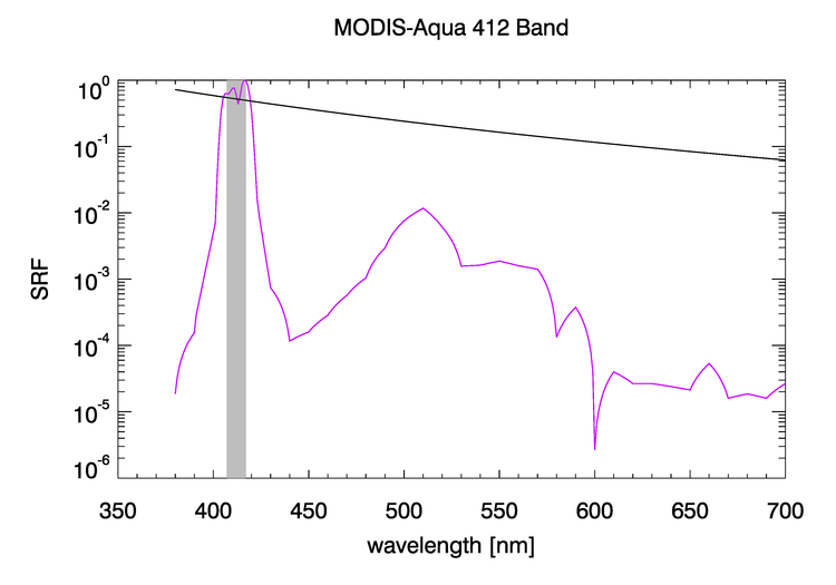
Figure 4 shows $R_{rs}\left(\lambda \right)$ as computed for Case 1 water using a model of the type developed in Morel and Maritorena (2001) for $K_d\left(\lambda \right)$ and $R(\left(\lambda \right)$.

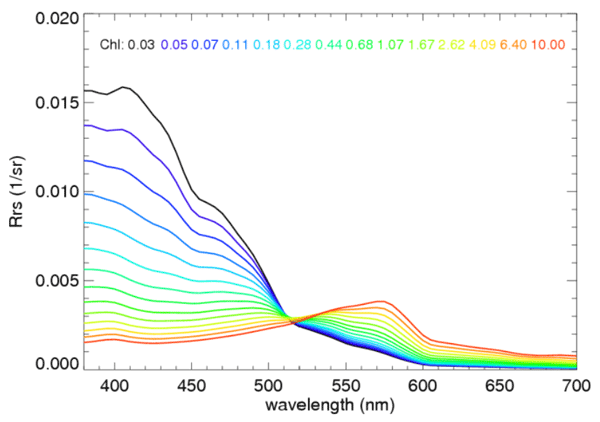
For each nominal sensor band labeled by ${\lambda }_i,i=1,...,N_{bands}$, and for each chlorophll value $Ch{l}_j,j=1,...,N_{Chl}$, the $R_{rs}\left(\lambda \right)$ spectra of Fig. 4 are used in equations of the form of (1) with appropriate integration limits to compute:

• $R_{rs}^{11}\left({\lambda }_i,Ch{l}_j\right)=$ The mean $R_{rs}$ over idealized 11-nm bandwidths (center wavelength $\pm 5$ nm) corresponding to the nominal satellite bands (as illustrated by the gray 412 nm band in Fig. 3)
• $R_{rs}^{full}\left({\lambda }_i,Ch{l}_j\right)=R_{rs}$ computed using the full spectral response function for the $i^{th}$ sensor band.
• The ratio

  $$r\left({\lambda }_i,Ch{l}_j\right)=\frac{R_{rs}^{11}\left({\lambda }_i,Ch{l}_j\right)}{R_{rs}^{full}\left({\lambda }_i,Ch{l}_j\right)}.$$

  (2)

Figure 5 illustrates the results of these calculations for the SeaWiFS nominal 555 nm band. This figure shows chlorophyll values only for $Chl\le 3mg{m}^{-3}$, which was felt to be the upper limit of reliability of the chlorophyll-based $R_{rs}\left(\lambda \right)$ model of Fig. 4. A similar figure can be drawn for each sensor band. If the chlorophyll concentration were known, a rearrangement of Eq. (2) and ratio curves like that of Fig. 4 could be used to compute the correction to the measured $R_{rs}^{full}$ for the $i^{th}$ band.

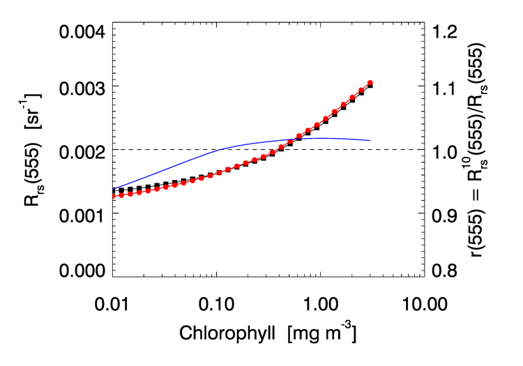
However, the chlorophyll concentration is not yet known. To proceed, the $r\left({\lambda }_i,Ch{l}_j\right)$ curves like the one shown by the blue line of Fig. 5 are used to compute correction factors $r\left({\lambda }_i\right)$ as functions of the ratio of the uncorrected $R_{rs}\left(490nm\right)$ to the uncorrected $R_{rs}\left(555nm\right)$. Each chlorophyll value shown in figures like 5 for the various bands gives a point like those shown in Fig. 6 for $r\left(555\right)$ vs. the uncorrected $R_{rs}\left(490\right)∕R_{rs}\left(555\right)$. A corresponding set of $r\left({\lambda }_i\right)$ points is computed for each band, but in each case as a function of $R_{rs}\left(490\right)∕R_{rs}\left(555\right)$. (This choice of the ratio of 490 to 555 nm for the independent variable traces back to SeaWiFS, for which these were the most trustworthy bands.) A best-fit function to the set of points so generated is then found for each of the $r\left({\lambda }_i\right)$ vs. $R_{rs}\left(490\right)∕R_{rs}\left(555\right)$ functions.

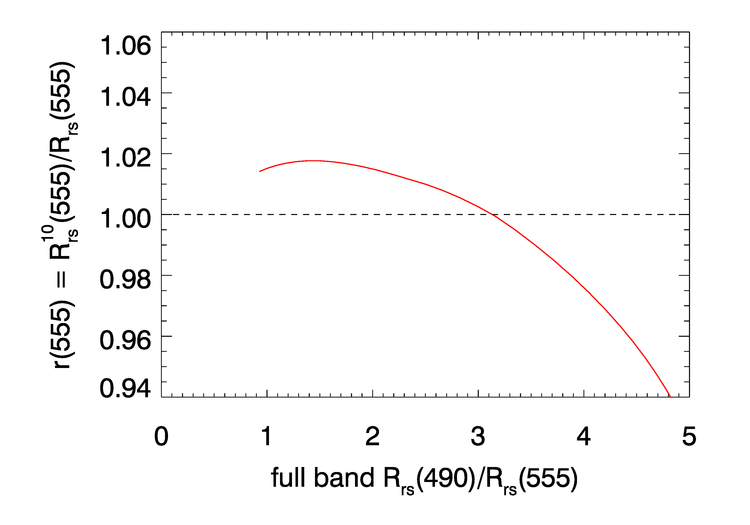
These functions are then used to apply the OOB correction to the measured $R_{rs}\left(555\right)$ values as follows. Given the measured full-band (uncorrected) $R_{rs}\left(i\right)$, the value of $R_{rs}\left(490\right)∕R_{rs}\left(555\right)$ is used to evaluate the functional fit to the points of Fig. 6 in order to obtain the correction to be applied to the $R_{rs}\left(555\right)$ value. The corresponding functions for the other bands are used to correct those bands. For example, the fit to $r\left(412\right)$ vs. $R_{rs}\left(490\right)∕R_{rs}\left(555\right)$ is used to correct the 412 nm band, and so on. If the $R_{rs}\left(490\right)∕R_{rs}\left(555\right)$ value is outside the range of the points used for the data fit as illustrated in Fig. 6, the value of the nearest point is used, rather than extrapolating with the fitting function beyond the range of the underlying data.

The $R_{rs}\left(i\right)$ functions were developed using a Case 1 model for $R_{rs}\left(\lambda \right)$ as shown in Fig. 4. Case 2 waters can have much different $R_{rs}\left(\lambda \right)$ spectra and therefore should have different OOB corrections. However, in practice, Case 2 waters have the same correction applied as for Case 1 waters.

A final comment is warranted regarding the use of this out-of-band correction when comparing satellite-derived and in-situ measurements of $R_{rs}$ (e.g, when doing vicarious calibration):

• If comparing a multispectral satellite band $R_{rs}$ with in an in situ multispectral measurement, perform the OOB adjustment to the satellite data. (Of course, an adjustment should also be made to the in situ values based on the relative spectral responses $SRF\left(\lambda \right)$ of the in situ radiometer.)
• If comparing a multispectral satellite band $R_{rs}$ with in an situ hyperspectral measurement that has been filtered with a 10 nm bandpass filter, perform the adjustment.
• If comparing a multispectral satellite band $R_{rs}$ with an in situ hyperspectral measurement that has not been filtered, do not perform the OOB adjustment to the satellite data. However, the hyperspectral in situ spectrum should processed using the satellite sensor $SRF\left(\lambda \right)$ spectra. That is, replace the spectrum used in integrals of the form of Eq. (1) with the hyperspectral $R_{rs}\left(\lambda \right)$.

Performing the OOB adjustment is the default for processing imagery at OBPG. Therefore, if a user wants to compare satellite data with unfiltered hyperspectral data as in the third bullet above, the standard Level 2 files cannot be used. The user would need to begin with the Level 1b TOA radiances, disable the OOB correction in the atmospheric correction software, and reprocess the TOA radiances to Level 2.