Page updated:
May 19, 2021
Author: Curtis Mobley
View PDF
Importance Sampling
As we saw on the previous Error Estimation page, the standard error of the mean in a Monte Carlo estimate depends on , where is the number of samples. In the present discussion, is the number of rays reaching a detector. In addition, we have seen that rays that are traced but do not intersect the detector—i.e., do not generate a sample of the underlying pdf—do not contribute to the answer and are wasted calculations.
The general topic of importance sampling considers ways to generate and trace rays so that more rays reach the detector, thus increasing and thereby reducing the statistical error in the estimated quantity, while simultaneously reducing the number of wasted rays.
Theory of Importance Sampling
Let be the probability distribution function for variable . The basic idea of importance sampling is to “over sample” the parts of the pdf that are most ”important,” i.e., those parts of the pdf that send rays in the direction of the detector. Those parts of the pdf that send rays (often called “photon packets” in the Monte Carlo literature) in directions away from the detector are under sampled. Thus more rays are sent towards the detector, which increases the number detected and therefore reduces the variance in the estimated quantity, and fewer are sent in directions that never reach the detector. However, this process samples the pdf in a biased or incorrect manner compared to the physical process being studied. To account for the biased sampling of the pdf, the weight of each ray is adjusted to keep the final answer correct.
Mathematically, importance sampling is described as follows. The mean of any function of random variable is by definition
where the integration is over the full range of (e.g., over 0 to if is the polar scattering angle). This can be rewritten as
is the biased pdf used to generate random values of , and is the weight given to each biased sample of . The weight is just the ratio of the unbiased to the biased pdfs. Note that the estimate of the mean of when sampled by the correct, unbiased pdf is the same as the estimate of the weighted function, , when sampled with the biased pdf . The estimate is thus unbiased, even though is biased. Because the sampling is done using a biased pdf, importance sampling is sometimes called biased sampling. However, the estimate of is still unbiased, even though the sampling uses a biased pdf. The term importance sampling is therefore preferred in recent literature.
If the biased pdf is chosen well, it will increase the number of detected rays and thereby reduce the error in the estimate. However, each detected ray will have a smaller weight, so that the product of more detected rays times a smaller weight for each remains the same as for a smaller number of higher weighted rays that would be generated by the original pdf. As we will see in the following numerical examples, this basic idea often works well. However, in practice, the biasing can sometimes be pushed to extremes and actually increase the error in the estimate.
Embedded Point Source Example
The first numerical example is based on Gordon (1987). This paper provides a good starting point for examining in detail the advantages and pitfalls of importance sampling.
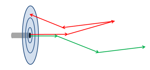
Gordon was interested in computing the irradiance pattern of upwelling light at the sea surface generated by an isotropic point source at some depth in the water. Figure 1 shows the geometry of his problem. The left panel of the figure shows an isotropic point source at depth emitting rays equally in all directions. For an isotropic source, half of all rays are emitted in downward directions. Few of those rays will be scattered in directions that eventually reach the sea surface. The same holds true for many rays emitted in upward, but nearly horizontal directions. Such rays are illustrated by the red arrows. Only rays emitted in nearly straight upward directions are likely to reach the surface and contribute to the estimate of upwelling irradiance as a function of radial distance away from the source location. The green arrow illustrates such a ray.
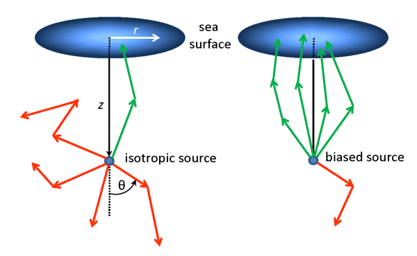
To increase the number of rays emitted almost straight upward, Gordon chose a biased pdf for the probability of emission of a ray at polar angle , measured from in the nadir direction ( is measured positive downward from the sea surface, and is measured from the direction). This isotropic emission is mathematically the same as isotropic scattering. Recall from the Introduction that the pdf for polar scattering angle is . Taking for the polar angle of emission and recalling that the phase function for isotropic scatter is shows that the pdf for the polar emission angle is . Gordon wished to have a biased pdf that would emit more rays into upward directions . There are many functions that could give such a behavior, but the one Gordon chose is
| (1) |
where is a parameter to be determined as described below. The weighting function is then
(Gordon did not say why he chose this particular function, nor did he give the value of used in his calculations.)
The right panel of Fig. 1 illustrates biased emission, with many more rays being emitted into upward directions and reaching the sea surface, and relatively few rays being emitted into downward directions.
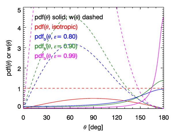
The red curves in Fig. 2 show the unbiased emission function , for which each emitted ray is given an initial weight of . The other curves show the biased functions and the angle-dependent initial weights for several values of . Note that as approaches 1, most rays are emitted at angles near , i.e. in near-zenith directions. However, rays emitted at angles near 180 deg are given very small weights, whereas the relatively few rays emitted in roughly horizontal and downward directions are given large weights (except for rays emitted near ).
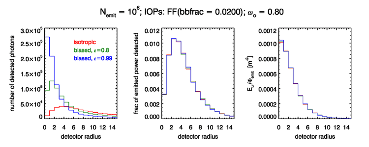
Monte Carlo simulations were performed for an unbiased isotropic source and for biased sources with various values. Figure 3 shows the results for a point source at optical depths below the surface and for water IOPs defined by a Fournier-Forand phase function with a backscatter fraction of 0.02 and an albedo of single scatter of . Independent runs were done for isotropic emission and for values of and 0.99 in Eq. (1). Each run had rays emitted by the source. The rays reaching the sea surface were tallied for a ring (or ”bullseye”) detector centered above the source and having equally spaced differences in ring diameters of in optical distance.
The left panel of the figure shows the number of rays received by each detector ring. For the isotropic source, at most about 40,000 rays were received by any ring (near radius = 5), and fewer than 10,000 rays were received by the innermost ring. As increases, the rays are emitted in a more and more vertical direction, and the numbers of rays received by the inner rings increase. The innermost ring received about 94,000 rays for and 270,000 rays for . We thus naively expect that the variance of the estimated irradiance in the innermost ring is improved by a factor of with , compared to unbiased isotropic emitting. Or, conversely, we can get the same number of detected rays for one-fifth of the emitted rays, i.e., for one-fifth of the computer time.
However, there is no free lunch. The outer rings, greater than about 5 or 6 optical distances in these simulations, received fewer rays with the biased emission than for isotropic emission. Thus the variance in the estimates of irradiance for the outer rings actually increases when using a biased source emission. This is simply because the biased near-zenith emission and subsequent near-forward scattering sends most of the rays towards the inner rings when nears 1.
The middle panel of the figure shows the fraction of the emitted power that is detected for each ring. Although the numbers of rays received by the rings varies according to the value of , the power received does not (except for statistical noise, which is almost unnoticeable in this figure). The right panel shows the irradiance received in each ring normalized to the total power emitted by the source, . This is just the values of the middle panel divided by the area of each ring. This panel corresponds to Fig. 6 in Gordon’s paper, except that the IOPs are different.
There is more to be learned from this simple example. Suppose we are interested only in the magnitude of the irradiance received at the ocean surface directly above the source. We might then consider only the power received by the innermost ring of the detector seen in the previous figure, i.e. detector radius in those plots.
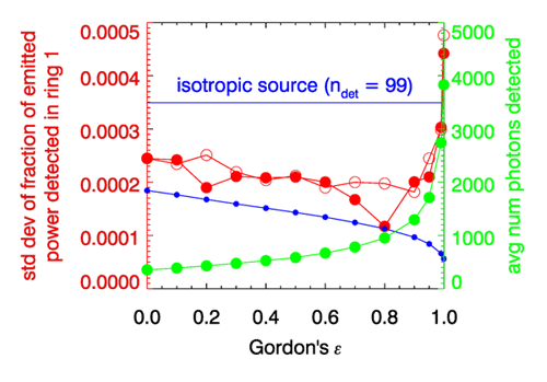
Consider the variance in the estimated fraction of the emitted power detected (i.e., of the surface irradiance, after dividing by the constant collection area) by the innermost ring of the previous figure, as a function of . Simulations were performed for isotropic emission and for values of from 0.0 to 0.999 (note that in Eq. 1 is not the same as isotropic emission). Each simulation comprised 100 runs with photo packets emitted for each run. The red dots in Fig. 4 show the standard deviation in the estimated value of the fraction of emitted power received by the innermost ring as computed from the values in each of the 100 runs. The open red circles show the corresponding results from an independent set of 100 runs, which started with a different seed for random number generation. Those two sets of points give a qualitative idea of the amount of statistical noise in these results. For isotropic emission an average of only 99 rays reached the detector out of the 10,000 emitted in each run (for the first set of runs with the first seed; for the second set the average was 101). The mean of the 100 runs was and the standard deviation was . When biased emission is used, the number of detected rays increases with as shown by the green dots and right-hand axis in the figure. The standard deviation decreases with increasing up to values around or 0.9. However, beyond the standard deviation beings to increase, and even becomes greater than for isotropic emission when , even though almost 4,000, or 40% of the emitted rays reach the detector. This seems to contradict the idea that increasing the number of detected rays reduces the variance.
It was already mentioned on the previous page on error estimation that the dependence of the standard deviation of an estimate on assumes that “all else is the same” in the simulation. In the present case, we are changing the physics of the simulation (namely the emission pattern of the source) by using a biased source, in which case all else is not the same. As was shown in the theory section, this change in physics does not affect the estimated mean value, but it does affect the variance of that estimate over many runs. The use of a biased emission pattern does increase the number of detected rays and thereby reduce the standard deviation of the estimated quantity, but only up to a point. When is very close to 1, only a very few rays are emitted in downward directions. However, those rays can have very large weights: for the maximum weight is 45.6. rays emitted within 10 deg of the zenith ( in Fig. 2) have weights less than 0.07, and those emitted within 5 deg of the zenith have weights less than 0.008. Thus the downward-emitted rays can have weights hundreds or even thousands of times larger than the vast majority upward-emitted rays. The large numbers of low-weight detected rays do reduce the error in the estimate. However, when is very close to 1, one of the downward-emitted but very-large-weight rays may occasionally be backscattered in just the right direction to hit the detector and make a large contribution to the fraction of the emitted power detected. Such rays are few in number, so their contribution fluctuates from simulation to simulation, and the difference of even a few rays may significantly changed the estimate. These rare rays then increase the standard deviation of the computed quantity, and the benefits of the biased source emission are lost.
The blue dots in Fig. 4 show the reduction in the standard deviation as expected due only to the increased numbers of detected rays, i.e. a dependence on . The actual improvement is less than the value that would be obtained if the runs were just emitting and detecting more rays for an isotropically emitting source (i.e., for the ”all else is the same” situation). Nevertheless, the reduction in the standard deviation is roughly a factor of two, which is significant for many applications.
Figure 5 shows the numbers of detected rays binned by the weights of the detected rays for three of the runs, and for and 0.8. For , the left panel shows that most of the detected rays have weights in the range of to 0.1. However, a very few (2, 4 and 5 ray packets in these particular runs) have weights between 1 and 10. One ray with a weight of 1 contributes as much to the estimated irradiance as 1000 rays with a weight of . The numbers of medium-weight rays are stable for the different runs, but the numbers of the highest-weight rays fluctuate greatly. The fluctuation in the number of high-weight rays begins to increase the variance for values very near 1. The numbers of very-low-weight rays also varies greatly from one run to the next, but those fluctuations have a negligible effect on the variance because the weights are so small. The right panel of this figure shows that for , most of the detected rays have weights in the range of 0.001 to 0.1, the numbers of rays in each bin is almost the same for each run, and there are no rays with weights greater than 1. Thus gives a stable number of medium-weight rays and a reduction in the standard deviation of the estimated detected weight, as desired. Note that in each case the estimate of the fraction of power received is , so the estimated mean is almost independent of .
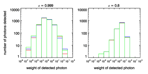
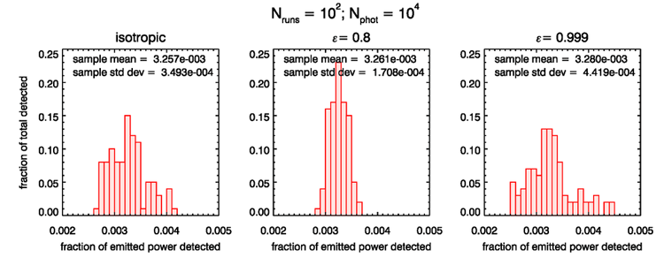
Figure 6 gives yet another view of this situation. The left panel shows the histogram of the 100 estimates of the fraction of emitted power detected by the innermost ring for isotropic emission. The middle panel shows a tighter histogram for , i.e., a reduced error in the estimate. The right panel shows the histogram for ; the spread is now wider and the error in the estimate has increased.
The behavior of the estimated error when doing importance sampling can be succinctly summed up as the tails of the distribution matter. That is to say, importance sampling can in many cases give more detected rays and a corresponding decrease in the error of the estimated quantity. However, the biasing can be pushed too far. In the present case, if is too close to 1, the rare but high-weight rays—those in the high-weight tail of the distribution of ray weights in Fig. 5—can overpower the reduction of variance obtained by the numerous but low-weight rays in the main part of the distribution of ray weights.
There is no general rule for determining how much biasing can be used or what value of a parameter like gives the minimum error in the estimated quantity. However, the broad near-minimum seen in Fig. 4 shows that any value of will give a better estimate than naive isotropic emission, and fortunately the exact value used is not critical. A suitable value of a biasing parameter such as must be determined by numerical experimentation for a particular class of problems. However, this effort is worthwhile if many simulations must be made and computer time or accuracy are critical.
Backscatter Example
Now consider an example of using importance sampling in the simulation of backscatter, as might be needed for the design and evaluation of an instrument to measure the backscatter coefficient . This example is inspired by the Monte Carlo simulations used in Gainusa Bogdan and Boss (2011), who did not use importance sampling.
The generic geometry for simulating a sensor is shown in Fig. 7. This figure illustrates a source emitting ray packets in a collimated beam. The distance a ray packet travels between interactions with the medium is randomly determined using the ray path length algorithm described in the Introduction of this chapter. Those ray packets are then scattered according to the chosen phase function , where is the polar scattering angle and is the azimuthal scattering angle. ray tracking is done by the ”Type 2” technique of the page on Ray Tracing. That is, at each scattering, the initial ray weight is multiplied by the albedo of single scattering , where is the scattering coefficient and is the beam attenuation coefficient. This accounts for energy loss due to absorption.
Oceanic phase functions are highly peaked in the forward scattering direction. Thus most ray packets undergo multiple forward scatterings and continue to travel away from the source and detectors. The green arrows in Fig. 7 illustrate such a ray trajectory. Only rarely will a ray be backscattered in just such a manner that it is eventually detected, as illustrated by the red arrows in the figure. For typical oceanic conditions, only 0.5 to 3% of rays are backscattered in any given interaction. For a spatially small detector, very few of the backscattered rays will actually intersect the detector. The end result is that almost every ray emitted from the source is wasted computation because the ray never reaches the detector.
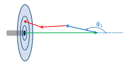
These simulations can be improved by use of importance sampling, as follows. The ray packets are emitted by the source according to whatever distribution is chosen (e.g., an idealized collimated point source or a beam profile and distribution of emitted directions that describes a particular light source such as an LED). Those rays travel an initial distance determined by the beam attenuation coefficient and the random number drawn. Then, on the first scattering only, the scattered direction is determined using a biased phase function that gives an increased number of backscattered rays. This “reverses” many of the initial rays, all of which are traveling away from the detector. Subsequent scatterings then use the normal phase function for the water body. This gives an increased number of ray packets traveling in the general direction of the detector, and thus an increased number of detected rays. This is illustrated in Fig. 8. The green arrow is the initial ray emitted by the source. The blue arrow is the first-scattered ray, whose direction is determined using the biased phase function. The red arrows are subsequent scatterings of the ray.
In oceanic simulations, the unbiased pdf is highly forward scattering. To reverse some of the initial rays, we use a biased pdf that enhances backscatter. The one-term Henyey-Greenstein (OTHG) phase function with asymmetric parameter ,
gives a convenient analytical phase function to use for . The parameter plays the same role as in the previous example. A value of gives isotropic scattering (50% backscatter); a negative gives more backscatter than forward scatter. Numerical investigations show that the results are not sensitive to the exact form of the biased phase function, so long as the biasing is not pushed to extremes (such as using in the OTHG, which gives 98% backscatter). Just as in the previous example, if the biasing is pushed too far, the small-angle forward-scattered rays have very large weights. The rare one of these rays that is subsequently backscattered (by normal scattering) into the detector gives a large fluctuation in the computed mean, which offsets the reduction in variance obtained by detecting many more low-weight rays.
The green curve of Fig. 9 shows a Fournier-Forand phase function with a backscatter fraction of ; this phase function is typical of ocean water and gives a good fit to the Petzold average-particle phase function. The red curve shows a OTHG phase function with , which gives a backscatter fraction of . When used as the biased phase function , this OTHG gives 40 times more backscattered rays at the first scattering event as does the Fournier-Forand phase function. The blue curve shows the corresponding weighting function . Note that the biased backscattered ray packets are given weights less than 0.1, whereas the very small angle forward scattered rays can have weights as large as 1000.
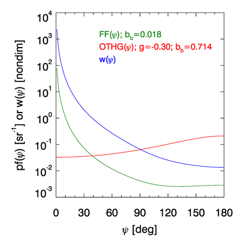
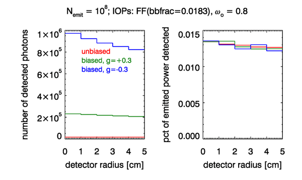
Figure 10 and Table 1 show example simulations with and without biased first scatterings. The target was an annular (“bullseye”) detector like the one in Fig. 7, but with five rings each of 1 cm radial width. This is similar to the proposed sensor design in Gainusa Bogdan and Boss (2011). The water properties were defined by a Fournier-Forand phase function with a backscatter fraction of 0.0183, which is shown in Fig. 9. The absorption coefficient was and the scattering coefficient was . The albedo of single scattering is then , which is typical of ocean waters at blue or green wavelengths. Three simulations were done: one without biased scattering and two with first scatterings biased with a OTHG phase functions with either or . The OTHG with has a backscatter fraction of , and has . The left panel of the figure shows the numbers of rays received by each detector ring; the right panel is the percent of emitted power received by each ring. Note that 12.9 times more rays reach the detector when biased first scattering is used with (green curve), and 52.6 times more for (blue curve) than for unbiased scattering (red curve). However, the fraction of emitted power received by the detector (over all 5 rings) remains the same, 0.0645%, to within less than 0.5% percent of Monte Carlo noise.
| First Scattering | Increase | % Emitted Power | |
| (all rings) | Factor | Detected (all rings) | |
| unbiased | 84,645 | — | 0.0648 |
| biased, | 1,093,114 | 12.9 | 0.0645 |
| biased, | 4,451,875 | 52.6 | 0.0642 |
Conversely, for a given number of rays detected, biased first scattering allows that number to be detected with fewer rays being emitted and traced to completion, i.e., with less computer time. For unbiased scattering, running the Monte Carlo code with unbiased scattering until 100,000 rays reached the detector (total over all 5 rings) required the emission of ray packets and a total run time of 6632 sec (on a 2.4 GHz PC). However, use of biased scattering with required emission of only rays, and a total run time of 105 seconds. The percent of emitted power that was detected was the same to within 3% in both cases, but the run time savings was a factor of 63.
[Additional pages on Monte Carlo topics such as forced collisions and backward ray tracing are under development.]
 See comments posted for this page and leave your own.