The Single-Scattering Approximation

As previously noted, exact analytical solutions of the RTE exist only for a few idealized and unphysical situations such as no scattering. There are, however, a few approximate analytic solutions. In pre-computer days these were useful computational tools. These approximate solutions are no longer needed for numerical computation, but they are still useful for isolating the most important processes governing light propagation in the ocean and can provide guidance in interpretation of radiometric data. This page develops one such solution: the single-scattering approximation (SSA). The next page discusses the related quasi-single scattering approximation (QSSA).

The Successive Order of Scattering Solution Technique

We begin with the optical depth form of the time independent, 1D (plane parallel geometry) RTE, which is Eq. (4) of the Scalar Radiative Transfer Equation page:

$$\begin{array}{llll}\hfill \mu \frac{dL\left(\zeta ,\mu ,\varphi ,\lambda \right)}{d\zeta }=& -L\left(\zeta ,\mu ,\varphi ,\lambda \right)& \hfill & \\ \hfill +& {\omega }_o\left(\zeta ,\lambda \right){\int \; <!--nolimits-->}_0^{2\pi }{\int \; <!--nolimits-->}_{-1}^{1}L\left(\zeta ,{\mu }^{\prime },{\varphi }^{\prime },\lambda \right)\tilde{\beta }\left(\zeta ;{\mu }^{\prime },{\varphi }^{\prime }\to \mu ,\varphi ;\lambda \right)d{\mu }^{\prime }d{\varphi }^{\prime }& \hfill & \\ \hfill +& \frac{1}{c\left(\zeta ,\lambda \right)}\Sigma \left(\zeta ,\mu ,\varphi ,\lambda \right).& \hfill & \end{array}$$ We next make a number of simplifications by assuming that

• The water is homogeneous, so that the IOPs do not depend on depth;
• The water is infinitely deep;
• The sea surface is level (zero wind speed);
• The sun is a point source is a black sky, so that the incident radiance onto the sea surface is collimated;
• There are no internal sources or inelastic scattering.

The RTE then becomes, for a given wavelength $\lambda$, which we henceforth drop for brevity,

$$\begin{array}{llll}\hfill \mu \frac{dL\left(\zeta ,\mu ,\varphi \right)}{d\zeta }=& -L\left(\zeta ,\mu ,\varphi \right)& \hfill & \\ \hfill +& {\omega }_o{\int \; <!--nolimits-->}_0^{2\pi }{\int \; <!--nolimits-->}_{-1}^{1}L\left(\zeta ,{\mu }^{\prime },{\varphi }^{\prime }\right)\tilde{\beta }\left({\mu }^{\prime },{\varphi }^{\prime }\to \mu ,\varphi \right)d{\mu }^{\prime }d{\varphi }^{\prime }.& \hfill \text{(1)}\end{array}$$

A powerful technique for solving differential equations is to attempt a power series solution in which higher order terms of the series are weighted by a powers of a parameter whose magnitude is less than 1. The higher order terms then contribute less and less to the sum that represents the solution. The albedo of single scattering, ${\omega }_o$, meets the requirement for an expansion parameter. We therefore attempt a solution of Eq. (1) of the form

$$\begin{array}{llll}\hfill L\left(\zeta ,\mu ,\varphi \right)=& \sum _{k=0}^{\infty }{\omega }_o^k{L}^{\left(k\right)}\left(\zeta ,\mu ,\varphi \right)& \hfill & \\ \hfill =& L^{\left(0\right)}\left(\zeta ,\mu ,\varphi \right)+{\omega }_o{L}^{\left(1\right)}\left(\zeta ,\mu ,\varphi \right)+{\omega }_o^2{L}^{\left(2\right)}\left(\zeta ,\mu ,\varphi \right)+\cdots & \hfill \text{(2)}\end{array}$$ The notation $L^{\left(0\right)}$ denotes radiance that is unscattered, $L^{\left(1\right)}$ is radiance from rays that have been scattered once, $L^{\left(2\right)}$ is radiance from rays that have been scattered twice, and so on. This is consistent with the interpretation of ${\omega }_o$ as the probability of ray survival in an interaction with matter, i.e., the probability that a ray will be scattered and not absorbed.

We now substitute Eq. (2) for the radiance into Eq. (1) to obtain

$$\begin{array}{llll}\hfill \mu & \left[\frac{d{L}^{\left(0\right)}}{d\zeta }+{\omega }_o\frac{d{L}^{\left(1\right)}}{d\zeta }+{\omega }_o^2\frac{d{L}^{\left(2\right)}}{d\zeta }+\cdots \right]& \hfill & \\ \hfill =& -\left[L^{\left(0\right)}+{\omega }_o{L}^{\left(1\right)}+{\omega }_o^2{L}^{\left(2\right)}+\cdots \right]& \hfill & \\ \hfill +& {\omega }_o{\int \; <!--nolimits-->}_0^{2\pi }{\int \; <!--nolimits-->}_{-1}^1\left[L^{\left(0\right)}+{\omega }_o{L}^{\left(1\right)}+{\omega }_o^2{L}^{\left(2\right)}+\cdots \right]\tilde{\beta }\left({\mu }^{\prime },{\varphi }^{\prime }\to \mu ,\varphi \right)d{\mu }^{\prime }d{\varphi }^{\prime }.& \hfill \text{(3)}\end{array}$$ We next group terms that have the same power of ${\omega }_o$:

$$\begin{array}{llll}\hfill & \left[\mu \frac{d{L}^{\left(0\right)}}{d\zeta }+L^{\left(0\right)}\right]& \hfill & \\ \hfill +{\omega }_o& \left[\mu \frac{d{L}^{\left(1\right)}}{d\zeta }+L^{\left(1\right)}-{\int \; <!--nolimits-->}_0^{2\pi }{\int \; <!--nolimits-->}_{-1}^1{L}^{\left(0\right)}\tilde{\beta }\left({\mu }^{\prime },{\varphi }^{\prime }\to \mu ,\varphi \right)d{\mu }^{\prime }d{\varphi }^{\prime }\right]& \hfill & \\ \hfill +{\omega }_o^2& \left[\mu \frac{d{L}^{\left(2\right)}}{d\zeta }+L^{\left(2\right)}-{\int \; <!--nolimits-->}_0^{2\pi }{\int \; <!--nolimits-->}_{-1}^1{L}^{\left(1\right)}\tilde{\beta }\left({\mu }^{\prime },{\varphi }^{\prime }\to \mu ,\varphi \right)d{\mu }^{\prime }d{\varphi }^{\prime }\right]& \hfill & \\ \hfill +\cdots & =0.& \hfill & \end{array}$$ This equation must hold true for any value of $0\le {\omega }_o<1$. Setting ${\omega }_o=0$ would leave only the first line of the equation, whose terms must sum to 0. Similarly, when ${\omega }_o\ne 0$, each group of terms multiplying a given power of ${\omega }_o$ must equal zero in order for the entire left side of the equation to sum to zero. We can therefore equate to zero the groups of terms in brackets multiplying each power of ${\omega }_o$. This gives a sequence of equations:

$$\begin{array}{lll}\hfill \mu \frac{d{L}^{\left(0\right)}}{d\zeta }=& -L^{\left(0\right)}& \hfill \text{(S0)}\\ \hfill \mu \frac{d{L}^{\left(1\right)}}{d\zeta }=& -L^{\left(1\right)}+{\int \; <!--nolimits-->}_0^{2\pi }{\int \; <!--nolimits-->}_{-1}^1{L}^{\left(0\right)}\tilde{\beta }\left({\mu }^{\prime },{\varphi }^{\prime }\to \mu ,\varphi \right)d{\mu }^{\prime }d{\varphi }^{\prime }& \hfill \text{(S1)}\\ \hfill \mu \frac{d{L}^{\left(2\right)}}{d\zeta }=& -L^{\left(2\right)}+{\int \; <!--nolimits-->}_0^{2\pi }{\int \; <!--nolimits-->}_{-1}^1{L}^{\left(1\right)}\tilde{\beta }\left({\mu }^{\prime },{\varphi }^{\prime }\to \mu ,\varphi \right)d{\mu }^{\prime }d{\varphi }^{\prime }& \hfill \text{(S2)}\end{array}$$ and so on. Note that because ${\omega }_o$ multiples the path integral term in Eq. (3), the path integrals in this sequence of equations always involve the radiance at one order of scattering less than the derivative term. We first solve Eq. (S0), which governs the unscattered radiance. The solution for $L^{\left(0\right)}$ then can be used in Eq. (S1) to evaluate the path integral, which becomes a source function for singly scattered radiance. After solving Eq. (S1) for singly-scattered radiance, $L^{\left(1\right)}$ can be used to evaluate the path function in Eq. (S2), and so on. This process constitutes the successive-order-of-scattering (SOS) solution technique.

Solution of Eq. (S0) for the unscattered radiance

To solve (S0) we need boundary conditions at the sea surface and bottom. Figure 1 reminds us that the incident unscattered radiance onto the sea surface, and transmitted into the water, is perfectly collimated because we have assumed that the sun is a point source in a black sky and the surface is level. In that figure, $E_{\perp }\left(0\right)$ denotes the irradiance measured just below the sea surface on a plane that is perpendicular to the direction of photon travel (denoted by the red dashed line), and ${𝜃}_{sw}$ is the Sun’s zenith angle in the water after refraction by the level surface.

---

---

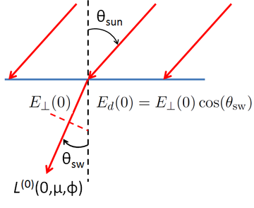
Recalling the Dirac delta function, we can write the unscattered radiance just below the surface as

$$L^{\left(0\right)}\left(0,\mu ,\varphi \right)=E_{\perp }\left(0\right)\delta \left(\mu -{\mu }_{sw}\right)\delta \left(\varphi -{\varphi }_{sw}\right),$$

(BC1)

where $\left({\mu }_{sw},{\varphi }_{sw}\right)$ is the direction of the Sun’s beam in the water. The two delta functions, which together have units of $s{r}^{-1}$, “pick out” the direction of the Sun’s beam; the unscattered radiance is zero in all other directions. Note that integrating this radiance over all downward directions to compute the downwelling plane irradiance gives

$$\begin{array}{llll}\hfill E_d\left(0\right)=& {\int \; <!--nolimits-->}_0^1{\int \; <!--nolimits-->}_0^{2\pi }{E}_{\perp }\left(0\right)\delta \left(\mu -{\mu }_{sw}\right)\delta \left(\varphi -{\varphi }_{sw}\right)\mu d\mu d\varphi & \hfill & \\ \hfill =& E_{\perp }\left(0\right){\mu }_{sw}& \hfill & \end{array}$$ as expected.

It is assumed that the incident solar irradiance is given, so Eq. (BC1) is the boundary condition on $L^{\left(0\right)}\left(\zeta ,\mu ,\varphi \right)$ at the sea surface (i.e., in the water at depth $\zeta =0$). We are assuming that the water is infinitely deep and source free, so the radiance must approach 0 at great depth. The boundary condition at the bottom is thus

$$L^{\left(0\right)}\left(\zeta ,\mu ,\varphi \right)\to 0as\zeta \to \infty .$$

(BC2)

We can now solve Eq. (S0) subject to boundary conditions (BC1) and (BC2). Rewriting (S0) as

$$\frac{d{L}^{\left(0\right)}\left(\zeta \right)}{L^{\left(0\right)}\left(\zeta \right)}=-\frac{d\zeta }{\mu }$$

and integrating from depth 0 to $\zeta$, corresponding to radiances $L^{\left(0\right)}\left(0\right)$ and $L^{\left(0\right)}\left(\zeta \right)$ respectively, gives

$${\left.ln{L}^{\left(0\right)}\right|}_{L^{\left(0\right)}\left(0\right)}^{L^{\left(0\right)}\left(\zeta \right)}={\left.-\frac{{\zeta }^{\prime }}{\mu }\right|}_0^{\zeta }$$

or

$$\begin{array}{lll}\hfill L^{\left(0\right)}\left(\zeta ,\mu ,\varphi \right)=& L^{\left(0\right)}\left(0,\mu ,\varphi \right)e^{-\zeta ∕\mu }& \hfill \text{(4a)}\\ \hfill =& E_{\perp }\left(0\right)\delta \left(\mu -{\mu }_{sw}\right)\delta \left(\varphi -{\varphi }_{sw}\right)e^{-\zeta ∕\mu }.& \hfill \text{(4b)}\end{array}$$

Solution (4a) is simply the Lambert-Beer law: the initial unscattered radiance decays exponentially with optical depth. Using (BC1) to rewrite the radiance at the surface gives (4b), which will be the convenient form for solution of (S1) below. Equation (4b) also shows explicitly that the unscattered radiance is 0 except in direction $\left({\mu }_{sw},{\varphi }_{sw}\right)$. The exponential forces the radiance to 0 as the depth increases, so that (BC2) is satisfied. Thus our solution satisfies both the surface and bottom boundary conditions and thus constitutes a complete solution of the two-point boundary value problem for unscattered radiance. This solution gives the contribution of unscattered radiance to the total radiance.

Solution of Eq. (S1) for the singly scattered radiance

The first step in solving (S1) is to evaluate the scattering term using the solution for $L^{\left(0\right)}$. To do this we use (4b) to get

$$\begin{array}{llll}\hfill & {\int \; <!--nolimits-->}_0^{2\pi }{\int \; <!--nolimits-->}_{-1}^1{L}^{\left(0\right)}\left(\zeta ,{\mu }^{\prime },{\varphi }^{\prime }\right)\tilde{\beta }\left({\mu }^{\prime },{\varphi }^{\prime }\to \mu ,\varphi \right)d{\mu }^{\prime }d{\varphi }^{\prime }& \hfill & \\ \hfill =& {\int \; <!--nolimits-->}_0^{2\pi }{\int \; <!--nolimits-->}_{-1}^1{E}_{\perp }\left(0\right)\delta \left({\mu }^{\prime }-{\mu }_{sw}\right)\delta \left({\varphi }^{\prime }-{\varphi }_{sw}\right)e^{-\zeta ∕{\mu }^{\prime }}\tilde{\beta }\left({\mu }^{\prime },{\varphi }^{\prime }\to \mu ,\varphi \right)d{\mu }^{\prime }d{\varphi }^{\prime }& \hfill & \\ \hfill =& E_{\perp }\left(0\right)e^{-\zeta ∕{\mu }_{sw}}\tilde{\beta }\left({\mu }_{sw},{\varphi }_{sw}\to \mu ,\varphi \right).& \hfill \text{(5)}\end{array}$$ This result shows how much of the unscattered radiance reaches depth $\zeta$ and then gets scattered into the direction of interest $\left(\mu ,\varphi \right)$. In other words, the unscattered radiance is a local (at depth $\zeta$) source term for singly scattered radiance.

All quantities on the right hand side of Eq. (5) are known from the given IOPs and surface boundary condition. We can therefore proceed with the solution of (S1) for the singly scattered radiance $L^{\left(1\right)}$. The equation to be solved is

$$\mu \frac{d{L}^{\left(1\right)}}{d\zeta }+L^{\left(1\right)}=E_{\perp }\left(0\right)e^{-\zeta ∕{\mu }_{sw}}\tilde{\beta }\left({\mu }_{sw},{\varphi }_{sw}\to \mu ,\varphi \right),$$

(6)

where the right hand side is now a known function of depth. There is no incident scattered radiance from the sky because the sun’s collimated beam is all unscattered light. Thus the boundary conditions for Eq. (6) are

$$L^{\left(1\right)}\left(0,\mu ,\varphi \right)=0and{L}^{\left(1\right)}\left(\zeta ,\mu ,\varphi \right)\to 0as\zeta \to \infty .$$

(7)

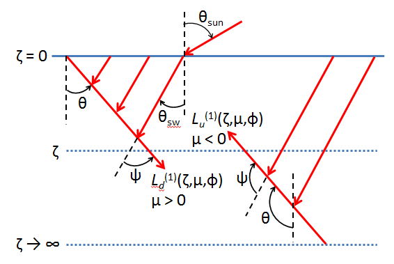
Figure 2 shows that the singly scattered downwelling radiance at depth $\zeta$ comes only from above depth $\zeta$, and that the upwelling radiance at $\zeta$ comes only from depths below $\zeta$. We can thus consider the downwelling, $L_d^{\left(1\right)}\left(\zeta ,\mu ,\varphi \right)$, and upwelling, $L_u^{\left(1\right)}\left(\zeta ,\mu ,\varphi \right)$, radiances separately. We can integrate from the surface down to $\zeta$ to compute $L_d^{\left(1\right)}$, and we can integrate from $\zeta$ to $\infty$ to compute $L_u^{\left(1\right)}$.

---

---

If you were paying attention in your undergraduate differential equations class, you recognize Eq. (6) as an ordinary differential equation with constant coefficients, which can be solved by means of an integrating factor. Multiplying Eq. (6) for downwelling radiance by $\frac{1}{\mu }{e}^{\zeta ∕\mu }$ (the integrating factor) gives

$$\begin{array}{llll}\hfill \frac{1}{\mu }{e}^{\zeta ∕\mu }\left[\mu \frac{d{L}_d^{\left(1\right)}\left(\zeta \right)}{d\zeta }+L_d^{\left(1\right)}\left(\zeta \right)\right]=& \frac{1}{\mu }{e}^{\zeta ∕\mu }\left[E_{\perp }\tilde{\beta }{e}^{-\zeta ∕{\mu }_{sw}}\right]& \hfill & \\ \hfill \frac{d}{d\zeta }\left[L_d^{\left(1\right)}\left(\zeta \right)e^{\zeta ∕\mu }\right]=& \frac{E_{\perp }\tilde{\beta }}{\mu }exp\left[\left(\frac{1}{\mu }-\frac{1}{{\mu }_{sw}}\right)\zeta \right].& \hfill \text{(8)}\end{array}$$ Now integrating from depth 0 to $\zeta$, where the radiances are $L_d^{\left(1\right)}\left(0\right)$ and $L_d^{\left(1\right)}\left(\zeta \right)$, respectively, and recalling that $L_d^{\left(1\right)}\left(0\right)=0$ by the upper boundary condition (7) gives

$$L_d^{\left(1\right)}\left(\zeta \right)e^{\zeta ∕\mu }=\frac{E_{\perp }\tilde{\beta }}{\mu }\frac{1}{\left(\frac{1}{\mu }-\frac{1}{{\mu }_{sw}}\right)}\left[exp\left(\frac{1}{\mu }-\frac{1}{{\mu }_{sw}}\right)\zeta -1\right],$$

provided that $\mu \ne {\mu }_{sw}$. Recalling that $E_d\left(0\right)=E_{\perp }\left(0\right){\mu }_{sw}$, the preceding equation can be rewritten as

$$L_d^{\left(1\right)}\left(\zeta ,\mu ,\varphi \right)=E_d\left(0\right)\tilde{\beta }\left({\mu }_{sw},{\varphi }_{sw}\to \mu ,\varphi \right)\frac{1}{{\mu }_{sw}-\mu }\left[e^{-\zeta ∕{\mu }_{sw}}-e^{-\zeta ∕\mu }\right].$$

(9)

For the special case of $\mu ={\mu }_{sw}$ but $\varphi \ne {\varphi }_{sw}$, so that the scattering angle is nonzero, Eq. (8) reduces to

$$\frac{d}{d\zeta }\left[L_d^{\left(1\right)}\left(\zeta \right)e^{\zeta ∕{\mu }_{sw}}\right]=\frac{E_{\perp }\tilde{\beta }}{{\mu }_{sw}}$$

which integrates to

$$\begin{array}{llll}\hfill L_d^{\left(1\right)}\left(\zeta ,{\mu }_{sw},\varphi \right)=& E_{\perp }\tilde{\beta }\left({\mu }_{sw},{\varphi }_{sw}\to {\mu }_{sw},\varphi \right)\frac{\zeta }{{\mu }_{sw}}{e}^{-\zeta ∕{\mu }_{sw}}& \hfill & \\ \hfill =& E_d\left(0\right)\tilde{\beta }\left({\mu }_{sw},{\varphi }_{sw}\to {\mu }_{sw},\varphi \right)\frac{\zeta }{{\mu }_{sw}^2}{e}^{-\zeta ∕{\mu }_{sw}}.& \hfill \text{(10)}\end{array}$$ The second form results from $E_d\left(0\right)=E_{\perp }\left(0\right){\mu }_{sw}$, which was derived above.

The direction of $\mu ={\mu }_{sw}$ and $\varphi ={\varphi }_{sw}$ is the case of no scattering, so there is no singly scattered radiance.

We next compute the upwelling radiance at $\zeta$ by integrating Eq. (6) from $\zeta$ to $\infty$, keeping in mind that now $\mu =cos𝜃<0$ since $𝜃$ is measured from 0 in the nadir direction. The integration gives (writing $\mu =-\left|\mu \right|$ to emphasize the negativity of $\mu$)

$$\begin{array}{llll}\hfill & {\left[L_u^{\left(1\right)}\left({\zeta }^{\prime }\right)e^{-{\zeta }^{\prime }∕\left|\mu \right|}\right]}_{{\zeta }^{\prime }\to \infty }-L_u^{\left(1\right)}\left(\zeta \right)e^{-\zeta ∕\left|\mu \right|}=& \hfill & \\ \hfill & \frac{E_{\perp }\tilde{\beta }}{-\left|\mu \right|}\frac{1}{\left(\frac{1}{-\left|\mu \right|}-\frac{1}{{\mu }_{sw}}\right)}\left\{{\left[exp\left(\frac{1}{-\left|\mu \right|}-\frac{1}{{\mu }_{sw}}\right){\zeta }^{\prime }\right]}_{{\zeta }^{\prime }\to \infty }-exp\left(\frac{1}{-\left|\mu \right|}-\frac{1}{{\mu }_{sw}}\right)\zeta \right\}& \hfill & \end{array}$$ Both limits as ${\zeta }^{\prime }\to \infty$ are zero. The result can be rewritten as

$$L_u^{\left(1\right)}\left(\zeta \right)=E_d\left(0\right)\tilde{\beta }\left({\mu }_{sw},{\varphi }_{sw}\to \mu ,\varphi \right)\frac{1}{{\mu }_{sw}-\mu }{e}^{-\zeta ∕{\mu }_{sw}}.$$

(11)

Assembling the SSA solution

Recalling from Eq. (2) that the SSA is given by

$$L^{\left(SSA\right)}\left(\zeta ,\mu ,\varphi \right)=L^{\left(0\right)}\left(\zeta ,\mu ,\varphi \right)+{\omega }_o{L}^{\left(1\right)}\left(\zeta ,\mu ,\varphi \right),$$

we can assemble $L^{\left(SSA\right)}$ from the pieces computed in Eqs. (4a) and (9-11):

$$\begin{array}{lll}\hfill L_d^{\left(SSA\right)}\left(\zeta ,\mu ,\varphi \right)=& L^{\left(0\right)}\left(0,{\mu }_{sw},{\varphi }_{sw}\right)e^{-\zeta ∕{\mu }_{sw}}& \hfill \text{(12)}\\ \hfill & if\mu ={\mu }_{sw}and\varphi ={\varphi }_{sw}& \hfill & \\ \hfill L_d^{\left(SSA\right)}\left(\zeta ,\mu ,\varphi \right)=& {\omega }_o{E}_d\left(0\right)\tilde{\beta }\left({\mu }_{sw},{\varphi }_{sw}\to {\mu }_{sw},\varphi \right)\frac{\zeta }{{\mu }_{sw}^2}{e}^{-\zeta ∕{\mu }_{sw}}& \hfill \text{(13)}\\ \hfill & if\mu ={\mu }_{sw}but\varphi \ne {\varphi }_{sw}& \hfill & \\ \hfill L_d^{\left(SSA\right)}\left(\zeta ,\mu ,\varphi \right)=& {\omega }_o{E}_d\left(0\right)\tilde{\beta }\left({\mu }_{sw},{\varphi }_{sw}\to \mu ,\varphi \right)\frac{1}{{\mu }_{sw}-\mu }\left[e^{-\zeta ∕{\mu }_{sw}}-e^{-\zeta ∕\mu }\right]& \hfill \text{(14)}\\ \hfill & if\mu >0and\mu \ne {\mu }_{sw}& \hfill & \\ \hfill L_u^{\left(SSA\right)}\left(\zeta ,\mu ,\varphi \right)=& {\omega }_o{E}_d\left(0\right)\tilde{\beta }\left({\mu }_{sw},{\varphi }_{sw}\to \mu ,\varphi \right)\frac{1}{E_{\perp }\left(0\right){\mu }_{sw}-\mu }{e}^{-\zeta ∕{\mu }_{sw}}& \hfill \text{(15)}\\ \hfill & if\mu \le 0& \hfill & \end{array}$$ Equations (12)-(15) constitute the SSA solution to the RTE. This solution is seen, for example, in Gordon (1994), where it is presented without derivation.

It is easy to show that

$$\underset{\mu \to {\mu }_{sw}}{lim}\frac{1}{{\mu }_{sw}-\mu }\left[e^{-\zeta ∕{\mu }_{sw}}-e^{-\zeta ∕\mu }\right]=\frac{\zeta }{{\mu }_{sw}^2}{e}^{-\zeta ∕{\mu }_{sw}},$$

(16)

in which case Eq. (14) reduces to Eq. (13), which was derived independently as a special case of the depth integration.

It must be remembered that the SSA rests upon a number of simplifying assumptions. In particular, the input sky radiance was collimated. The delta functions in direction then made evaluation of the scattering path function in Eq. (5) easy. This would not be the case for any other sky radiance distribution, or for a non-level sea surface. Likewise, the assumption of infinitely deep water removed any bottom effect.

The SSA will be a good approximation to actual radiances only if the higher order terms in the Eq. (2) are negligible. This means that ${\omega }_o$ must be sufficiently small, but how small? Figure 3 compares $L_u^{\left(SSA\right)}$ and $L_d^{\left(SSA\right)}$ with radiances computed by HydroLight for nadir- and zenith-viewing radiances. The sun was at 42 deg, which gives the in-water solar zenith angle of ${𝜃}_{sw}=30$ deg or ${\mu }_{sw}=0.866$. This gives a scattering angle of $\psi =30$ deg for $L_d^{\left(SSA\right)}$ and $\psi =150$ deg for $L_u^{\left(SSA\right)}$. The Petzold “average-particle” phase function) was used, for which $\tilde{\beta }\left(\psi =30\right)=0.08609$ and $\tilde{\beta }\left(\psi =150\right)=0.002365s{r}^{-1}$. HydroLight includes all orders of multiple scattering, so comparison of its radiances with the SSA values shows the importance of multiple scattering. The HydroLight runs modeled the SSA conditions as closely as possible, the difference being that the SSA is for one exact direction and HydroLight computes nadir and zenith radiances as averages over polar caps with a 5 deg half angle, and the sun’s direct beam in water is spread out over a quad from $𝜃=$ 25 to 35 deg. The HydroLight runs set $E_d\left(inair\right)=1.028W{m}^{-2}s{r}^{-1}$ so that $E_d\left(0\right)=1.0W{m}^{-2}s{r}^{-1}$.

---

---

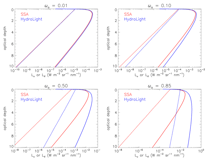
Figure 3 shows that for ${\omega }_o=0.01$ the agreement between the SSA and HydroLight is very good. The HydroLight values are slightly higher than the SSA values because there is still a small multiple scattering contribution to the total radiance even at very small ${\omega }_o$ values. For ${\omega }_o=0.1$ the SSA still gives good results near the sea surface but differs from the multiple scattering solution by a factor of 3 at 10 optical depths. For ${\omega }_o=0.85$, which is typical of blue and green wavelengths in ocean waters, the SSA upwelling radiance is a factor of five too small even at the surface, and the SSA radiances are off by orders of magnitude at large optical depths. Thus, as expected, we see that the SSA is of little use in optical oceanography because multiple scattering almost always dominates underwater radiance distributions at visible wavelengths.

We end the SSA discussion by noting that Walker (1994) has carried the SOS solution through second order scattering. His development requires a good bit of mathematical masochism and results in a much more complicated set of equations, which can be seen in his Section 2-6. There is little need for such approximations given the ease of numerical solution of the RTE to include all (in HydroLight) or at least many (in Monte Carlo models) orders of multiple scattering, and without any of the assumptions required for the analytic evaluation of the path integrals in the SSA. Perhaps the greatest value of the SSA solution is that it can be used to check numerical models when ${\omega }_o$ is small.