Classification Schemes

Taxonomies of Water Types

The classification of natural waters into optical water types, as with many other taxonomies, is done in order to generalize and systematize the science of ocean color. Arnone et al. (2004), in a review paper on water mass classification, credits the Secchi disk (invented around 1865) as the first quantitative optical instrument that has been used to measure water transparency and hence provided the ability to differentiate water mass based on their optical properties. Classification schemes that are based on water color are primarily based on absorption (as scattering contributes to intensity but less to color).

The most common classification schemes for water types are based on

• The human eye: visually compare the water color to the color of a standard color sample (Forel-Ule color scale)
• Analysis of AOP spectra (Jerlov water types)
• The relative importance of Chlorophyll in determining the optical properties of the water (Case 1 vs. Case 2)
• Analysis of inherent optical properties (ternery diagrams)

Human-eye-based Classifications: The Forel-Ule Color Classification

The Forel-Ule Scale is a method to approximately determine the color of bodies of water. Different inorganic compounds with standard formulas are used to produce a color palette with twenty one fluid vials covering blue to green to brown. The analysis consists of finding the vial whose color best matches the color of the water body; the result is an index from 1 to 21. The method is often used in conjunction with the Secchi disk and is included in data bases such as (NOAA’s World Ocean Database. The method was developed in the 1890s by Francois-Alphonse Forel and William Ule. Although now replaced by instruments for quantitative work, the Forel-Ule color measurements are still of interest because of the ease of making measurements and the large database of historical observations, which has value for studies of long-term changes in ocean ecosystems (e.g., Wernand (2011)). There is now even a smart-phone app for making Forel-Ule measurements. Figure 1 shows the use of a Forel-Ule color scale to determine the color of the ocean by visually determining the closest match of the water color to one of the 21 Forel-Ule colors.

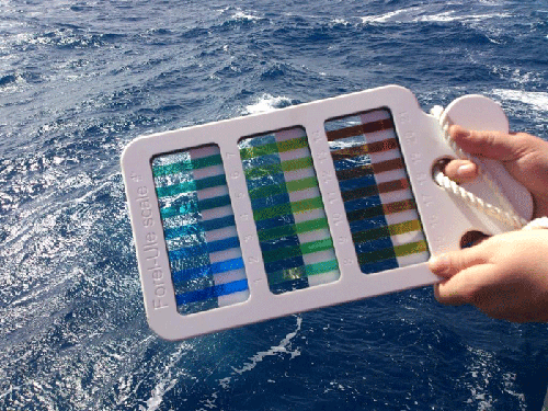
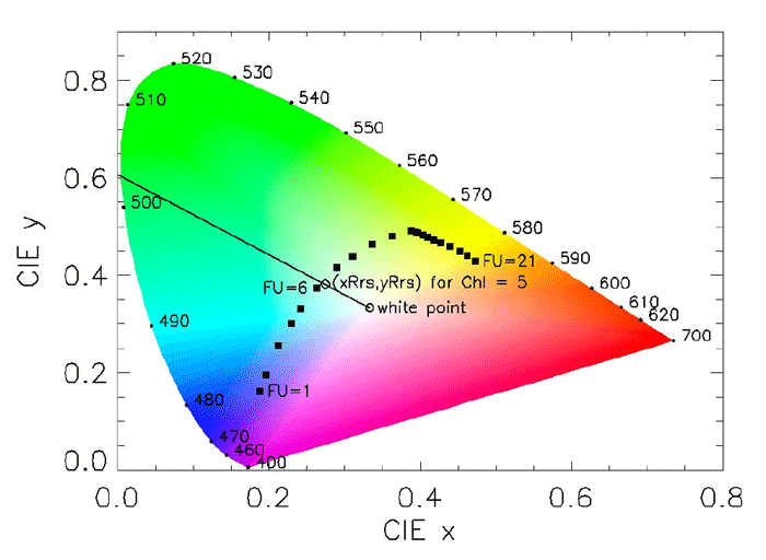
Figure 2 shows the locations of the 21 Forel-Ule colors on a CIE chromaticity diagram. The open circle is the white point. The open diamond is the CIE color of the remote-sensing reflectance $R_{rs}$ as calculated by HydroLight using the “new Case 1” IOP model with a chlorophyll concentration of $5mg{m}^{-3}$. The closest Forel-Ule value is 6.

Another comparative scale is the Hazen Platin-Cobalt-Scale adopted as the American Public Health Association (APHA) color scale (described in ASTM D1209,“Standard Test Method for Color of Clear Liquids (Platinum Cobalt Scale)”). It is based on diluting a standard stock solution (500ppm of PtCo) and finding the dilution whose color best matches the fluid compared.

Analysis of AOP Spectra: The Jerlov Classification

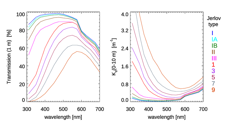
Jerlov (1968) introduced a classification of water bodies based on their spectral optical attenuation depth $z_k\equiv 1∕K_d$. Since ocean color is proportional to $1∕a\sim 1∕K_d$ these spectra are linked to the color observed. Jerlov discretized his observations into a set of five typical open-ocean spectra, labelled I, IA, IB, II, and III, and nine typical coastal spectra, labelled 1 to 9 (e.g., Tables XXVI and XXVII in Jerlov (1976); these data are linked here).

The Jerlov water types can be defined either by their irradiance transmission through a given thickness of water, or via the diffuse attenuation coefficient $K_d$ averaged over a given depth. The left panel of Fig. 3 shows the spectra defining the Jerlov types in terms of the irradiance transmission through 1 m of water. The right panel shows the corresponding spectra as the averages of $K_d$ over depths 0 to 10 m.

Morel (1988) gives a very approximate correspondence between the open-ocean Jerlov types and the chlorophyll concentration:

Solonenko and Mobley (2015) give tables relating the Jerlov water types to a consistent set of absorption and scattering coefficients (consistent in the sense that the IOPs, when used in HydroLight, generate $K_d$ spectra that correspond to the different Jerlov water types).

Importance of Chlorophyll versus Other Components: Case 1 versus Case 2 Water Types

Morel and Prieur (1977) described the spectral shape of $R=E_u∕E_d$ and its changes as separating two types of waters.

They found that “two extreme cases can be identified and separated. Case 1 is that of a concentration of phytoplankton high compared to other particles. In contrast, the inorganic particles are dominant in case 2. In both cases dissolved yellow substance is present in variable amounts. An ideal case 1 would be a pure culture of phytoplankton and an ideal case 2 a suspension of nonliving material with a zero concentration of pigments.”

Morel and Prieur emphasized that these ideal cases are not encountered in nature, and they suggested the use of high or low values of the ratio of pigment concentration to scattering coefficient as a basis for discriminating between Case 1 and Case 2 waters.

The definitions of Case1 and Case 2 have evolved over the years into the ones commonly used today (Gordon and Morel (1983), Morel (1988)):

• Case 1 waters are those waters whose optical properties are determined primarily by phytoplankton and co-varying colored dissolved organic matter (CDOM) and detritus degradation products.
• Case 2 waters are everything else, namely waters whose optical properties are significantly influenced by other constituents such as mineral particles, CDOM, or microbubbles, whose concentrations do not covary with the phytoplankton concentration.

In Case 1 waters, several changes occur as the pigment concentration increases:

1.

The $R$ values in the blue-violet region decrease progressively and a minimum is formed around 440 nm, which corresponds to the maximum absorption of chlorophyll. The maximum shifts toward 565-570 nm, which is the wavelength where simultaneously the absorption due to pigments is at its minimum and the absorption due to the water itself rapidly increases.

2.

The second maximum of absorption by chlorophyll a in vivo creates an $R$ minimum near 665 nm. This minimum is only slightly marked because the increase in absorption due to the presence of chlorophyll remains weak compared with the absorption due to water itself.

3.

At 685nm a second reflectance maximum appears due to fluorescence by chlorophyll superimposed on absorption/scattering interaction near the 676nm absorption band.

4.

A hinge point in $R$ values in the 560-640-nm band is observed with relatively little change as chlorophyll varies.

In Case 2 waters inorganic particles are relatively more dominant than phytoplankton. As the turbidity increases the following modifications appear:

1.

The reflectance values are generally higher than for case 1 throughout the spectrum and of a different shape. There is no longer, as in Case 1, a minimum at 440 nm. On the contrary, the curves become convex between 400 and 560 nm (inverted ’U’ shape rather than inverted ’V’). The maximum is flatter than in case 1, but located at the same wavelength, 560 nm.

2.

$R$ values become higher as turbidity increases. This is opposite of what was observed in Case 1, particularly for wavelengths above 550 nm.

3.

As a result of the flat shape of the $R$ curves, the dominant wavelength does not shift beyond 510 nm. These waters are blue-green or green with a bright and milky appearance due to the combined effects of high irradiance values and of low purity values.

Although the Case 1 versus Case 2 distinction has proven very useful, it can also be misleading. It must be understood that natural waters are not simply either Case 1 or Case 2; there is a continuous gradation of water optical properties (whether IOPs or AOPs) and their dependence on chlorophyll and other water constituents. It must also be remembered that “Case 1” and “Case 2” are not synonyms for “open ocean” and “coastal” waters.

Mobley et al. (2004) have even suggested that it is perhaps time to drop this type of binary classification as it sometimes obfuscates more than it helps. For example, the same water can be Case 1 for absorption but Case 2 for scattering (e.g., if the water contains non-absorbing but highly scattering mineral particles), or it can be Case 2 for absorption and Case 1 for scattering (e.g., if the water contains a high concentration of highly absorbing terrigenous CDOM, which does not covary with the chlorophyll, and which does not affect the scattering). Of course, water in the same area may be Case 1 during some time of the year and Case 2 in other times. Waters with similar chlorophyll concentrations may have large variations in ocean color in open ocean environment (e.g. Eastern Mediterranean vs. South Pacific gyre).

Ternery Diagrams

Ternary diagrams are a way to show the relative contributions of 3 variables to a total value using a 2D plot. In biological oceanography they are often used to show the relative contributions of absorption by phytoplankton, colored dissolved organic matter (CDOM), and non-algal particles (NAP) to the total absorption at a given wavelength (after subtracting out the water contribution). Figure 4 shows the layout of a ternary diagram to be used for this purpose. In that figure, the red triangle at the lower left represents all of the absorption being due to CDOM. The blue triangle at the lower right is the point for all absorption being due to NAP, and the green triangle at the top represents all absorption being due to phytoplankton. The red dotted lines are lines of constant CDOM contribution. That is, moving back and forth along one of the red lines leaves the CDOM contribution constant while the relative contributions of phytoplankton and NAP vary. Similarly, the green lines are lines of constant phytoplankon contribution, and the blue lines are “contours” of constant NAP contribution. (Of course, which side of the triangle corresponds to which component does not matter, nor does the “counterclockwise” versus “clockwise” direction of increasing values on each of the three axes.)

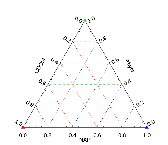
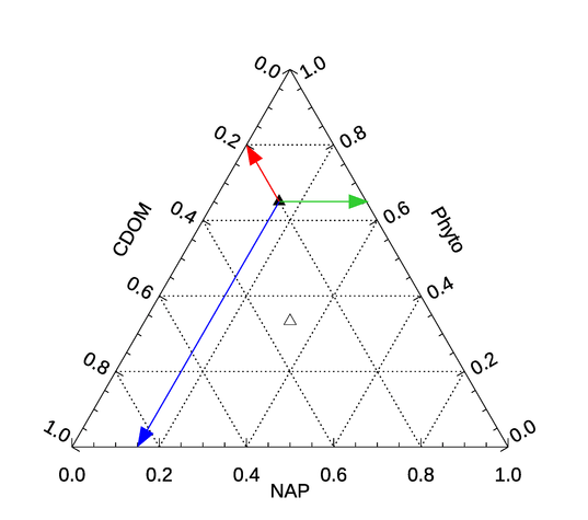
Figure 5 shows a point on a ternary diagram for the relative concentrations of phytoplankton as 0.65, CDOM as 0.2, and NAP as 0.15 of the total value. This point is shown by the black triangle. To determine the three contributions for a plotted point, follow lines parallel to the dotted lines of constant contributions back to the respective axes. This is illustrated by the red, green, and blue arrows, which are parallel to the red, green, and blue grid lines of Fig. 4. The open symbol at the centroid of the triangle shows the point corresponding to equal contributions by each of the three components.

An example of ternary diagrams applied to absorption is given in Figure 16 of Babin et al. (2003b). Those plots show the absorption contributions at various wavelengths for European coastal waters. Their diagram shows well how at different wavelengths different constituents (dissolved material, algae and non-algal particles) dominate absorption.

Other Classification Schemes

The preceding discussion has outlined the most commonly used classification schemes for natural waters. However, a number of other classifications have been developed and used for various applications. Representative schemes have been based on

• Cluster Analysis of $R_{rs}$ spectra: Eleveld et al. (2017), Mélin and Vantrepotte (2015), Prasad and Agrawal (2016), Wei et al. (2016)
• Fuzzy Logic Classification of $R_{rs}$ spectra: Moore et al. (2001), Moore et al. (2009), Moore et al. (2014):
• Principle Component Analysis/Empirical Orthogonal Functions: Lubac and Loisel (2007), Avouris and Ortiz (2019)
• Maximum wavelength of $R_{rs}$ spectra: Ye et al. (2016)
• Weighted means of $R_{rs}$ spectra: Vandermeulen et al. (2020)