Algorithm Introduction

The Level 2 pages of this chapter describe particular atmospheric correction algorithms, i.e., algorithms used to remove the various unwanted contributions to the top-of-the-atmosphere radiance. The next seven pages discuss, one by one, the various corrections made to the TOA radiance during the atmospheric correction process as implemented (as of 2016) by the NASA Ocean Biology Processing Group (OBPG) for processing satellite imagery. The philosophy of these pages is simply to show “Here is what is done. See the references for the historical development and scientiﬁc basis of the algorithms.”

The ﬁrst two pages show how to account for absorption and scattering by atmospheric gases. Sun glint and whitecap reﬂectances are then discussed, followed by the various aspects of correction for the eﬀects of atmospheric aerosols. Two pages then discuss the sensor-speciﬁc corrections for spectral out-of-band response and for polarization. The ﬁnal two pages describe methods for atmospheric correction that are sometimes used for airborne imagery or in situations for which the OBPG algorithms are not applicable.

For satellite imagery, the entire sequence of data processing beginning with the measurement of a TOA radiance and ending with the output of a geophysical product such as a global map of chlorophyll concentration is divided into a number of processing levels. These steps are deﬁned in Table 1. The OBPG atmospheric correction process described here takes the data from Level 1b to Level 2.

Table 1: Processing Levels. For further discussion see the NASA Ocean Color Products page.

Level	Deﬁnition
0	refers to unprocessed instrument data at full resolution. Data are in “engineering units” such as volts or digital counts.
1a	is unprocessed instrument data at full resolution, but with information such as radiometric and geometric calibration coeﬃcients and georeferencing parameters appended, but not yet applied, to the Level 0 data.
1b	refers to Level 1a data that have been processed to sensor units (e.g., radiance units). Level 0 data are generally not recoverable from level 1b data.
	Atmospheric correction is applied to Level 1b TOA radiance to create Level 2 data.
2	refers to derived geolocated, geophysical variables (e.g., normalized water-leaving reﬂectance ${[ρ_{w} (λ)]}_{N}^{e x}$ , chlorophyll concentration, $K_{d} (490 n m)$ , and AOT(865 nm)) at the same resolution and location as Level 1 data.
3	are variables mapped onto uniform space-time grids, often with missing points interpolated or masked, and with regions mosaiced together from multiple orbits to create large-scale maps, e.g. of the entire earth.
4	refers to results obtained from a combination of satellite data and model output (e.g., the output from an ocean ecosystem model), or results from analyses of lower level data (i.e., variables that are not measured by the instruments but instead are derived from those measurements).

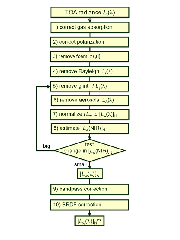
Figure 1 shows the sequence in which the various corrections are applied during the overall process.

Figure 1: Flowchart of the atmospheric correction process.

It is important to keep in mind that there are severe computational constraints on how atmospheric correction is performed on an operational basis. The MODIS-Aqua sensor, for example, collects about 1.4 terrabytes of data per day. The requirement to routinely process this amount of data (along with data from many other sensors) requires that various approximations be made in order to speed up the calculations. Some of the corrections require ancillary information such as sea level pressure, wind speed, and ozone concentration, which are not collected by ocean color sensors themselves. These ancillary data may be inaccurate or missing, in which case climatological values must be used. The quality of the ancillary information impacts the accuracy of the atmospheric correction. Table 2 shows some of the ancillary data and its sources as used by the various OBPG atmospheric correction algorithms.

Table 2: Ancillary data needed for atmospheric correction. Abbreviations: NCEP, National Centers for Environmental Prediction; OMI, Ozone Monitoring Instrument; TOMS, Total Ozone Mapping Spectrometer; SCIAMACHY, SCanning Imaging Absorption spectroMeter for Atmospheric CHartographY; GOME, Global Ozone Monitoring Experiment; Reynolds/NCDC, Reynolds analysis, National Climate Data Center; NCEI, NOAA National Centers for Environmental Information (previously NODC); NSIDC, National Snow and Ice Data. Center.

Data	Source	Use
atmospheric pressure	NCEP	Rayleigh correction
water vapor	NCEP	transmittance
wind speed	NCEP	Rayleigh, Sun glint, white caps
ozone concentration	OMI/TOMS	transmittance
$N O_{2}$ concentration	SCIAMACHY/OMI/GOME	transmittance
sea surface temperature	Reynolds/NCDC	seawater index of refraction and backscattering
sea surface salinity	NCEI World Ocean Atlas, Salinity Climatology	seawater index of refraction and backscattering
sea ice coverage	NSIDC	masking

The sea surface temperature and salinity are used to compute the water index of refraction and water backscattering coeﬃcient. Operationally, pixels are masked before atmospheric correction for only a few conditions, namely the presence of land or clouds, and saturation of the measured radiance. An attempt is made to process all other pixels. A separate mask is applied during atmospheric correction to pixels with too much Sun glint. Various ﬂags are incorporated into Level 2 and 3 data after the atmospheric correction process described below. These identify pixels that may have various problems such as sea ice contamination, turbid water, bottom eﬀects, or failed atmospheric correction. These ﬂags are listed at NASA Processing Flags. Other information on ﬂags is given in Chapter 6 of Patt et al. (2003). With the exception of Sun glint, applying masks and ﬂags is not a part of the atmospheric correction process per se, so this topic is not discussed here.

See comments posted for this page and leave your own.

Comments for Algorithm Introduction:

Loading Conversation

Non-absorbing Gases »