Non-absorbing Gases

This page describes the Rayleigh corrections made for non-absorbing gases. The next page describes the more complicated problem of absorbing gases.

A radiative transfer numerical model is used to solve the vector (polarized) radiative transfer equation for non-absorbing atmospheric gases only. The radiative transfer model includes atmospheric multiple scattering, polarization, and sea surface roughness modeled analytically by a Cox-Munk slope distribution with an added analytical wave shadowing function. The Cox-Munk slope distribution as used is azimuthally isotropic (no dependence on wind direction); therefore only the relative angle between Sun and viewing direction matters. This greatly simpliﬁes the Fourier decomposition seen in Eq. (3) of Wang (2002). The radiative transfer model is described in Ahmad and Fraser (1982).

Wind Speed and Surface Reﬂectance Eﬀects

Background sky reﬂectance by the rough sea surface is accounted for as part of the Rayleigh correction. Some sensors (CZCS, SeaWiFS, OCTS) can be tilted to avoid looking at glint near the Sun’s specular direction. Other sensors (MODIS, VIIRS, MERIS, OLI) do not tilt and therefore must account for specular reﬂection.

Wind speed and surface glint corrections are computed as described in Wang (2002): Run the numerical model to compute a look up table (LUT) of TOA Fourier components $L_{r}^{m} (λ, 𝜃_{s}, 𝜃_{v}, τ_{R o}, W)$ (his Eq. 3) for the following conditions:

The sensor wavelength bands (e.g., bands centered at 412, 443, 490, 510, 555, 670, 765, 865 for SeaWiFS). The radiative transfer model is run using band-averaged optical thicknesses (rather than running at high-wavelength resolution, and then averaging the $L_{r}$ values over the band response functions to get the nominal band values of $L_{r}$ for a particular sensor).
45 Sun zenith angles $𝜃_{s}$ from 0 to 88 deg by 2 deg
41 viewing nadir angles $𝜃_{v}$ from 0 to 84 deg by roughly 2 deg
Rayleigh optical thickness $τ_{R o}$ for standard sea level atmospheric pressure $P_{o} = 1013.25 h P a$ (1013.25 millibar).
8 wind speeds $W$ = 0, 1.9, 4.2, 7.5, 11.7, 16.9, 22.9 and 30.0 m/s. (These wind speeds correspond to convenient spacing in the mean square slopes of the sea surface according to the Cox-Munk equation $m s s = 0.00512 W$ : $m s s$ = 0.0, 0.01, 0.02, 0.04, 0.06,... for $W$ = 0, 1.9, 4.2, 7.5, 11.7, ....) Linear interpolation is used for values between these wind speeds.

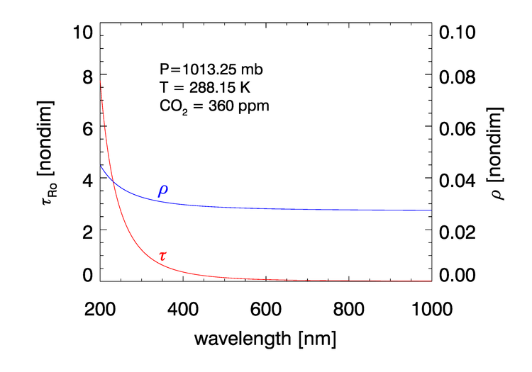
The Rayleigh optical thickness $τ_{R o} (λ)$ at 1 atmosphere of pressure, $P_{o}$ (1013.25 hPa), temperature of 288.15K, and a $C O_{2}$ concentration of 360 ppm is given by Eq. (30) of Bodhaine et al. (1999):

τ_{R o} (λ) = 0.0021520 (\frac{1.0455996 - 341.29061 λ^{- 2} - 0.90230850 λ^{2}}{1.0 + 0.0027059889 λ^{- 2} - 85.968563 λ^{2}}),

(1)

where $λ$ is in micrometers. These values and the corresponding Rayleigh depolarization ratio $ρ (λ)$ are shown in Fig. 1. (At the scale of this ﬁgure, the Bodhaine values are almost indistinguishable from the values given by the formula of Hansen and Travis (1974) (see Eq. (15) of Bodhaine et al. (1999)), which were used in earlier calculations.)

Figure 1: The Rayleigh optical thickness and depolarization ratio based on Bodhaine et al. (1999).

The Rayleigh LUTs for $L_{r}$ contain the $I, Q$ and $U$ Stokes vector components in reﬂectance units, as a function of wind speed and geometry. The Stokes vector $V$ component for circular polarization is assumed to be zero. There is a separate LUT for each wavelength.

During image correction, the wind speed $W$ for a given pixel comes from NCEP 1 deg gridded data, interpolated to the image pixel.

Pressure Eﬀects

The Rayleigh optical thickness at the time of the observation depends on the number of atmospheric gas molecules between the sea surface and the top of the atmosphere. The number of molecules is directly proportional to the sea-level pressure $P$ . Thus the Rayleigh optical thickness at any pressure $P$ is given by

τ_{R} (P, λ) = \frac{P}{P_{o}} τ_{R o} (P_{o}, λ) .

The TOA $L_{R}$ is then computed by Eq. (5) of Wang (2005) and subsequent equations:

L_{R} [τ_{R} (P, λ)] = L_{R} [τ_{R} (P_{o}, λ)] \frac{1 - exp [- C (λ, M) τ_{R} (P, λ) M]}{1 - exp [- C (λ, M) τ_{R} (P_{o}, λ) M]},

(2)

where

M = \frac{1}{cos 𝜃_{s}} + \frac{1}{cos 𝜃_{v}}

(3)

is the geometric air mass factor for the total path through the atmosphere. $C (λ, M)$ is a coeﬃcient that is determined so that Eq. (2) gives the best ﬁt to $L_{R} [τ_{R} (P, λ)]$ as computed by an extremely accurate atmospheric radiative transfer model when run for values of sea level pressure $P \neq P_{o}$ . Numerical simulations show that this coeﬃcient can be modeled as

\begin{array}{l} C (λ, M) = & a (λ) + b (λ) ln (M) \\ a (λ) = & - 0.6543 + 1.608 τ_{R} (P_{o}, λ) \\ b (λ) = & 0.8192 - 1.2541 τ_{R} (P_{o}, λ) . \end{array}

Non-absorbing Gases

Wind Speed and Surface Reﬂectance Eﬀects

Pressure Eﬀects

Comments for Non-absorbing Gases: