Physics of Absorption

Collin Roesler and Curtis Mobley contributed to this page.

This page introduces the physical processes that lead to absorption of light by an atom or molecule. Beginning with a few basic concepts from quantum mechanics, we qualitatively show why a molecule like chlorophyll has an absorption spectrum that is unique to that molecule.

Quantum Mechanics Terminology

The terminology of quantum mechanics can be confusing. Physicists tend to speak of quantum numbers (principle, azimuthal, magnetic, and spin); chemists talk about orbitals and shells and subshells. Both groups are describing the same thing in ways that best fit their respective needs. There are also various graphical ways to represent the arrangement and energies of electrons in an atom or molecule.

An electron orbital refers to the size and shape of the three-dimensional spatial region where an electron is likely to be found, say with $\ge 90\%$ probability, at any moment. The term emphatically does not imply that electrons buzz around nuclei in well defined orbits like planets going around the Sun. Such an image from classical physics is completely wrong as a way to visualize atoms. If an analogy is needed, it is perhaps permissible to think of “orbital” as loosely corresponding to “energy level.” However, in many cases, different orbitals correspond to the same energy, in which case the energy levels are said to be “degenerate.”

The principal quantum number $n=1,2,3,...$ describes the overall physical size of the orbital; i.e., the average distance of an electron from the nucleus. The azimuthal or angular quantum number $l=0,1,...,n-1$ describes the shape of the orbital. The magnetic quantum number $m=-l,-l+1,...,0,1,...,l$ describes orbital’s orientation in space (originally with respect to an externally applied magnetic field, hence the name). The spin quantum number s can have values of $+1∕2$ or $-1∕2$ and defines the direction (usually called “up” or “down”) of the component of an electron’s intrinsic angular momentum (spin) along the direction of an external field. Nature does not allow two electrons in the same atom to have the same set of quantum numbers $n,l,m,s,$ which is known as the Pauli exclusion principle.

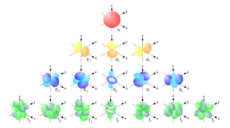
Orbitals with the same value for the principal quantum number form a shell. Shells are often labeled with letters starting at K (for historical reasons rooted in spectroscopy). Electrons with a principal quantum number of $n=1$ are in the K shell; electrons with $n=2$ are in the L shell; those with $n=3$ are M-shell electrons, and so on. Subshells are orbitals in the same shell that have the same magnetic quantum number. Subshells are labeled s for $l=0$, p for $l=1$, d for $l=2$, and so on for f, g, h,... in that order (again, these letters arose in spectroscopy and stood for “sharp,” “principal,” and “diffuse” spectral lines). Thus an electron with quantum numbers $n=1,l=0$ is said to be in a 1s orbital (spoken as ”one ess”); an electron in a 2p (two pee) orbital has $n=2,l=1$. s orbitals are spherically symmetrical. The three p orbitals consist of 2 lobes. Four of the five d orbitals are four-lobed somewhat like a clover leaf, and one is lobed with a torus around its “equator.” There is no spatial orientation for spherically symmetric s orbitals, but p orbitals can have their lobes oriented along the $x$, $y$, or $z$ axes of some coordinate system, and so on for the other non-spherical orbitals. Figure 1 shows a qualitative visualization of orbital shapes for s, p, d, and f orbitals.

Because of the attraction between a negative electron and the positive nucleus, the physically smallest, spherically symmetric orbital, which on average over time has the electron closest to the nucleus, has its electron most tightly bound to the nucleus. This is the 1s orbital. The corresponding ground state energy is represented as a negative value (usually in units of electron volts, eV; $1eV\approx 1.60\times 10^{-19}J$). To remove a ground-state electron from the molecule requires this amount of energy to “raise” the electron to 0 binding energy, i.e., no binding to the nucleus. Moving an electron from the ground state to an orbital with $n>1$ moves the electron further from the nucleus and therefore requires energy to overcome the electrical attraction. Similarly, an electron in a 2p orbital will have more energy than one in a 2s orbital, because a 2p electron spends more time further from the nucleus that does a 2s electron. Finally, a particular orbital can hold at most two electrons, with spin quantum numbers of $s=\pm 1∕2$ (the Pauli exclusion principle). Note that the s orbital label is not to be confused with the $s$ spin quantum number.

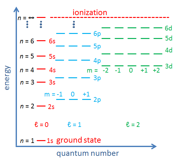
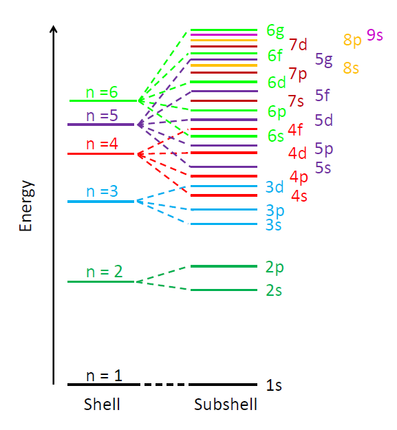
The allowed electron energy levels in an atom or molecule are often displayed on a diagram with binding energy on the y axis and the azimuthal and magnetic quantum numbers on the x axis. Such diagrams are sometimes called Jablonski diagrams. Figure 2 shows the conceptual layout of an energy level diagram with electron quantum numbers and orbitals labeled. The exact values of the energy levels for a given atom or molecule can be computed from the laws of quantum mechanics. Figure 3 shows another common way to display electron energy levels.

The previous discussion refers to the quantum numbers for individual electrons in an atom or molecule. In multi-electron atoms it is also common to write quantum numbers for the total quantum state of all electrons in the atom or molecule. That is, each electron in the molecule has an azimuthal quantum number, which represents its angular momentum with respect to the nucleus. Angular momentum is a vector, so the total angular momentum of all electrons is the vector sum of the angular momentum vectors of the individual electrons, computed using the quantum mechanical rules for adding quantized angular momenta. The resulting total angular momentum quantum number is denoted by a capital letter $L$ with values of $L=0,1,2,...$. Likewise, the vector sum of the spin angular momenta of the individual electrons gives the spin quantum number for the whole atom or molecule, which is denoted by $S$. For atoms with an even number of electrons, the resulting possible values for $S$ are 0, 1, 2,.... For atoms with an odd number of electrons, the resulting $S$ values can be 1/2, 3/2, 5/2, .... In the same way, the total orbital and total spin angular momentum vectors can be combined to obtain a total angular momentum, described by a new quantum number $J$, whose values are either integral (for an even number of electrons) or half-integral (an odd number of electrons) from $|L-S|$ to $L+S$. The z component of the total angular momentum is specified by quantum number $M$, which can have either integral (if $J$ is integral) or half-integral (if $J$ is half-integral) values from $-J$ to $+J$. This gives four total or “spectroscopic” quantum numbers $L,S,J,M$.

When the $L$ quantum number is 0, 1, 2, 3,..., the atomic or molecular quantum state is labeled with letters S, P, D, F,..., in analogy with s, p, d, f,... for electron states with $l=0,1,2,3,....$ The value of $2S+1$ is written as a preceding superscript, and the $J$ value as a following subscript: ${}^{2S+1}{L}_J$, e.g ${}^1{\text{S}}_0$, ${}^2{\text{P}}_{1∕2}$, ${}^3{\text{P}}_0$, and so on (read as “singlet ess zero”, “doublet pee one half”, “triplet pee zero”, and so on). Again note the difference in the S state labeling the value of the quantum number $L$ vs the total spin quantum number $S$. The value of quantum numbers $L$ and $M$ are not to be confused with the L and M electron shells corresponding to electron principal quantum numbers $n=2$ and $n=3$. Note also that a 3p electron state is different from a ${}^3\text{P}$ atomic or molecular state. As we said, the notation can be confusing.

Fortunately this is already more that we need to know for the following qualitative discussion of absorption spectra. However, this material will be needed later, for example in understanding fluorescence. In any case, the basics of quantum-mechanical terminology are mentioned here in hope of minimizing confusion when the lower-case and upper-case notations are seen elsewhere. The excellent ChemWiki and the atomic spectroscopy chapter of J. B. Tatum’s online Stellar Atmospheres give more detailed but still qualitative presentations of these matters, which are treated in their full quantum-mechanical glory in texts on quantum physics and chemistry.

Absorption

For the present, it is sufficient to know that the electrons in an atom or molecule have very specific energies—that is, the allowed electron energies are quantized. This physical reality is reflected mathematically in the discrete (integer or half-integer) values of the quantum numbers introduced above.

Recall that light is a propagating electromagnetic field. For the moment, we can think (rather naively) of a photon as a region of space with a propagating and rapidly fluctuating electric field. If the electric field is oscillating with a frequency $\nu$ (units of Hertz, i.e. cycles per second or $s^{-1}$), then the photon has energy

where $h$ is Planck’s constant, $c$ is the speed of light, and $\lambda$ is the wavelength (in a vacuum).

As a photon approaches an atom or molecule, the electrons in the atom or molecule begin to “feel” the photon’s electric field. Let $E_1$ be the energy of an electron in one of the subshells, and let $E_2$ be the higher energy of one of the subshells that does not contain an electron. If the photon frequency corresponds to the energy difference between these two energy levels, i.e., if

then there is a chance that the electron will absorb the photon and use the photon’s energy to “jump” from its current subshell with energy $E_1$ to the vacant higher-energy subshell with energy $E_2=E_1+h\nu$. The atom or molecule is then said to be in an excited energy state. The time scale for this absorption-excitation process is about $10^{-15}s$. This is the fundamental way that matter absorbs light. If the photon frequency does not correspond to any of the subshell energy differences, then the light cannot be absorbed and the photon continues on its way.

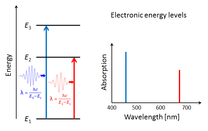
Figure 4 illustrates three electron energy levels of a molecule. Which shells or subshells these levels correspond to in a particular molecule is irrelevant for the present discussion. The usual situation for a molecule is that the lower-energy subshells are all occupied by electrons. It is then likely that visible light will raise one of the outermost (highest energy) electrons to an unoccupied energy level. (Raising an electron from the 1s shell to a higher shell typically requires ultraviolet light.) The red and blue arrows in the left panel of the figure represent electrons absorbing blue- and red-wavelength photons and jumping from a low energy level to higher ones. The right panel of the plot shows the corresponding absorption lines in the absorption spectrum of the molecule.

The probabilities for photon absorption are generally different for different transitions. Thus some absorption lines will be “stronger” than others. This is represented by a higher magnitude of the blue absorption line in the right-hand plot. In emission—the reverse of absorption—a photon is emitted when an electron falls from an excited state to an unoccupied lower energy level. In that case, some emission lines will be “brighter” than others. The visual nature of these emission lines was the origin of the spectroscopic labels of “sharp,” “principle,” “diffuse,” and “fine,” which were later related to the quantum numbers and orbitals as described above.

The situation of Fig. 4 is typical of atoms and simple molecules in near isolation (e.g., in gases). However, the situation becomes more complicated for molecules containing many atoms. In addition to the electron energy levels, molecules also have vibrational modes, as illustrated in Table 1. The blue spheres in the animations represent atoms attached to the side of a larger molecule. These vibrational modes also have quantized energy levels. That is, the molecules can vibrate only at specific frequencies, which are determined by the molecule’s structure and the atoms involved.

---

Symmetrical Stretching	Asymmetrical Stretching	Rotating
Twisting	Wagging	Scissoring

Table 1: Molecular vibration modes. Animations from WikiMedia, e.g. symmetrical stretching

---

It usually requires less energy to excite a vibrational mode than to excite an electron from one subshell to another. The spacing between the quantized vibrational energy levels is thus less than between electron orbitals. A quick calculation is instructive. Molecular vibrational frequencies fall in the $10^{12}$ to $10^{14}{s}^{-1}$ range. For $\nu =10^{13}{s}^{-1}$, $\lambda =c∕\nu$ gives a wavelength of $30\mu m$, which is in the mid-infrared. Thus infrared light can excite a molecule from one vibrational mode to another (with no change in the electronic energy level). The corresponding vibrational energy difference is $\Delta E_v=h\nu =hc∕\lambda =0.04eV$. (A useful relation for these sorts of calculations is $hc\approx 1.24eV\mu m$.)

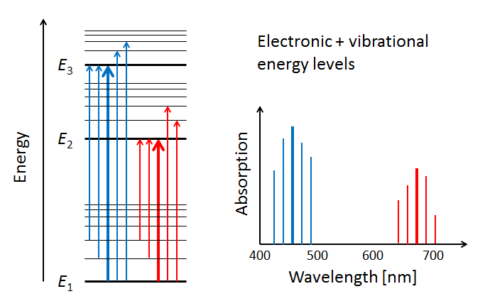
Now suppose that we are interested in an electronic transition corresponding to a blue wavelength of $440nm=0.440\mu m$. The corresponding electronic energy shift is $\Delta E_e=h\nu =hc∕\lambda =2.82eV$. If the vibrational modes now allow energy levels that are equal to the electronic transition $\pm$ a vibrational level, the energy shift can be $\Delta E_e\pm \Delta E_v$. The corresponding wavelengths are then $\lambda =hc∕\left(\Delta E_e\pm \Delta E_v\right)$, which in the current example gives $\lambda =0.434$ and $0.446\mu m$, or a wavelength shift of 6 nm to either side of the 440 nm electronic transition line.

The thin horizontal lines in the left panel of Fig. 5 represent the additional molecular energy levels when both electronic and vibrational levels are included in the energy diagram. The thin blue and red arrows in the left panel illustrate how the presence of vibrational modes allows for more possible electronic transitions to occur in the wavelength neighborhoods of the electronic transitions between subshells. These transitions add more spectral lines to the absorption spectrum, as shown by the thin lines in the right-hand panel.

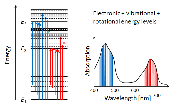
In addition to the vibrational modes, molecules also have rotational modes. That is, the entire molecule can rotate about an axis with some frequency, which is again quantized. Exciting a molecule from one rotational mode to another typically requires very little energy (in the $10^{-3}$ to $10^{-6}eV$ range), so that microwave radiation ($\lambda$ in the millimeter to meter range) is adequate. When the additional quantized energy states associated with rotational modes are included in the energy diagram, the allowed energy levels become very closely spaced, as illustrated by the dashed lines in the left panel of Fig. 6. The corresponding changes in absorption line wavelengths are in the sub-nanometer range when compared to electronic or electronic-vibrational transitions. The net result of having electronic, vibrational, and rotational modes is that the resulting molecular absorption spectrum is such a dense collection of absorption lines that it appears as a continuous function of wavelength when measured by instruments with spectral responses greater than a nanometer.

We have now seen in a qualitative way how absorption spectra like those of chlorophyll arise. The final comment to make is that the absorption spectrum of chlorophyll $a$, for example, will be slightly different when measured in vivo (in a living cell) vs in vitro (literally “in glass,” i.e. after extraction from a cell). The reason is that the environment of the chlorophyll molecule effects how it can vibrate and rotate. Thus different environments change the allowed energy bands somewhat, and thus change the shape of the absorption curve.