Autocovariance Functions: Numerical Example

This page gives a numerical example of the Wiener-Khinchin theorem, which leads into the details of how to sample autocovariance functions so that the resulting variance spectra meet the needs for surface generation.

The blue curve of Panel (a) in Fig. 1 plots the one-sided Pierson-Moskowitz spectrum (Eq. 2 of the Wave Variance Spectra: Examples page) for wind speed of $U_{10}=5m{s}^{-1}$. Using this spectrum, surfaces are generated at $N=1024$ points over a region of length $L=100m$. Note that $N$ is a power of 2 as required for the use of the fast Fourier transform algorithm. The spacing of these points is at intervals of $\Delta x=L∕N=0.0944m$. The red dot at ${\nu }_1=1∕L=0.011∕m$ is the fundamental frequency. The point at ${\nu }_{N∕2}=1∕\left(2\Delta x\right)=5.121∕m$ is the Nyquist spatial frequency. The green vertical ticks show the locations of the remaining $N-2$ points, which are evenly spaced at intervals of $\Delta \nu =0.011∕m$.

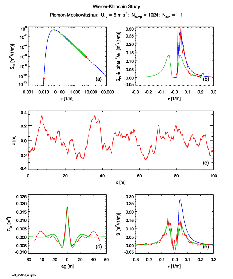
These discrete samples of the variance spectrum are then used as described on the Spectra to Surfaces: 1D page to create a random realization of the sea surface $z\left(r\right)$ at $N$ points. One such surface, generated for a particular sequence of random variables, is shown in Fig. 1(c). The periodogram of this surface, computed via Eqs. (2) and (3) of the Surfaces to Spectra: 1D page and Eq. (4) of the Spectra to Surfaces: 1D page, is shown in red in Fig. 1(b). The blue curve in this panel is the one-sided spectrum ${\mathcal{𝒮}}_{1s}\left(\nu \right)$ of Panel (a), replotted for reference. The statistical noise in the periodogram is Gaussian distributed about the theoretical ${\mathcal{𝒮}}_{1s}\left(\nu \right)$. These three panels of the figure are the essentially the same as the figure on the Spectra to Surfaces: 1D page; the only difference is that the sequence of random numbers used to generate the surface is different and linear axes are used for the upper-right panel.

Equation (3) of Autocovariance Functions: Theory page applied to the $z\left(r\right)$ of Panel (c) gives the autocovariance shown in red in Panel (d). This curve contains statistical noise. To obtain a theoretical curve for comparison, the Pierson-Moskowitz spectrum was sampled at 2048 points to insure coverage of most of the spectrum. The discrete Wiener-Khinchin theorem (Eq. 10 of the Autocovariance Functions: Theory page) was then used to obtain the autocovariance from the discretely sampled spectrum:

Here the DFT was computed via Eq. (8) of the Fourier Transforms page. Note that the discrete spectrum ${\mathcal{𝒮}}_{2s}\left(u\right)$ was obtained by sampling the continuous spectral density at the desired $\nu$ values and then multiplying by the appropriate bandwidth. Because ${\mathcal{𝒮}}_{2s}\left(u\right)$ is a real and even function of ${\nu }_u$, its Fourier transform is also real and even. The result is shown as the green curve in this Panel (d). Equation (5) of the Spectra to Surfaces: 1D page gives the total variance of $⟨z^2⟩=0.0197m^2$ for $U_{10}=5m{s}^{-1}$. The numerical result obtained by sampling ${\mathcal{𝒮}}_{2s}\left(\nu \right)$ and taking the inverse Fourier transform as just described gives $C_{zz}\left(0\right)=⟨z^2⟩=0.0178m^2$.

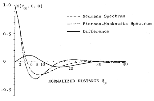
Latta and Bailie (1968) analytically computed the autocorrelation of the Pierson-Moskowitz spectrum in temporal form, but the result is a formula of horrible complexity consisting of the sum of five slowly converging infinite series, the terms of which are themselves are products of infinite series. That paper plots the numerically evaluated result in terms of an unspecified but normalized temporal lag, which makes comparison with the present results for spatial lag quantitatively impossible. However, de Boer (1969) obtained the spatial covariance of the Pierson-Moskowitz spectrum in the form of integrals of Bessel functions, which also require careful numerical evaluation. Figure 2 shows their result for the autocovariance function of waves in the down-wind direction. Their plot is in terms of a nondimensional normalized lag distance ${\xi }_N=\left(2g∕U^2\right)\ell$. The green curve of Fig. 1(d) has a minimum of $-0.0063m^2$ at $\ell =\pm 7.96m$. This translates to an autocorrelation of -0.31 at a normalized lag of ${\xi }_N=6.3$. These value are in reasonable agreement with the minimum seen in Fig. 2, keeping in mind that the curves in that figure were themselves generated on a 1960’s era computer by difficult numerical integrations of unknown accuracy. The agreements for the variance and the location and magnitude of the minimum indicate that the numerically computed $C_{zz}^{PM}\left(\ell \right)$ is probably correct for all lags. (This numerical calculation will be verified again with greater accuracy in the discussion of the Horoshenkov spectra below, for which the exact autocovariance is known.)

Taking the DFT of the green curve in Fig. 1(d) should give the two-sided spectrum ${\mathcal{𝒮}}_{2s}\left(\nu \right)$ corresponding to the one-sided spectrum plotted in Panel (a). The green curve in Panel (e) of that figure shows the result (after dividing by the finite bandwidth, as mentioned previously), which is indeed one-half of the one-sided spectrum ${\mathcal{𝒮}}_{1s}\left(\nu \right)$ (shown in blue). This provides a check on the correctness of a round-trip Fourier transform.

Taking the DFT of the red curve in Panel (d) gives a sample estimate of ${\mathcal{𝒮}}_{2s}\left(\nu \right)$, which is shown in red in Panel (e). This curve has statistical noise, but it visually appears to be distributed about the theoretical value given by the green curve.

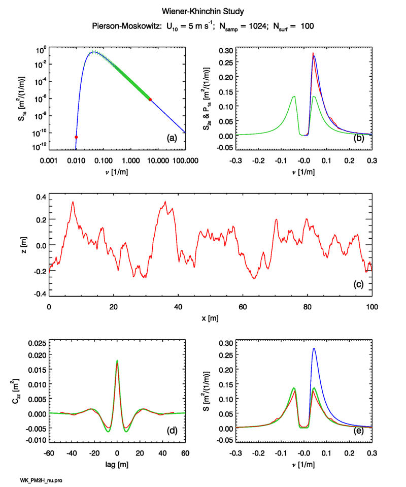
The statistical noise inherent in any single random realization of the sea surface and its autocovariance can be reduced by averaging the results from many surface realizations. Figure 3 is the same as Fig. 1, except that $N_{surf}=100$ independent surfaces are generated. This reduces the statistical noise by a factor of $1∕\sqrt{100}$. The red curve in Panel (b) shows the ensemble average periodogram for the 100 surfaces. It is clear that the average periodogram is in excellent agreement with the theoretical variance spectrum, except for a small amount of remaining statistical noise.

The red curve of Panel (d) is the average autocovariance for the 100 surfaces. This curve is much closer to the theoretical (green) curve than the autocovariance for the single surface of Fig. 1(d). The DFT of this average autocovariance is shown by the red curve in Panel (e). Again, this curve has much less noise and is closer to the (green) theoretical spectrum.

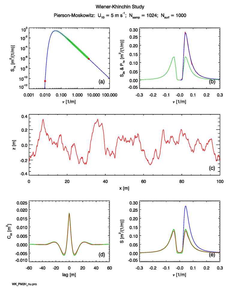
The statistical noise in the ensemble averages can be made arbitrarily small by averaging more and more surfaces. Figure 4 shows that averages for 1,000 surfaces have noise levels in the periodogram, autocovariance, and spectrum derived from the autocovariance, that are almost unnoticeable at the scale of the figures.