Page updated:
February 13, 2021
Author: Curtis Mobley
View PDF
Absorbing Gases
, , , and have negligible absorption at the visible and NIR wavelengths relevant to ocean color remote sensing. However, , , , and have absorption bands in the visible and NIR. The and bands can be avoided by judicious choice of sensor bands, as shown in Fig. 1 for the MODIS bands. However, as seen in Figs. 2 and 3, and have broad, concentration-dependent absorption bands that cannot be avoided. It is therefore necessary to account for absorption by these two gases.
The concentrations of absorbing gases are usually measured as column concentrations, i.e., the number of molecules per unit area, or as the equivalent in Dobson units. One Dobson unit refers to a layer of gas that would be thick at standard temperature and pressure, or about . 1000 DU = 1 atm-cm; that is, 1000 DU is the number of molecules that would give a layer of gas 1 cm thick at a pressure of one atmosphere.
![]()
![]()
![]()
For optically thin absorbing gases that are high in the atmosphere ( in particular), it is possible to correct for absorption using just the geometric air mass factor computed by
| (1) |
because scattering is not significant. However, for gases near the surface ( in particular), multiple scattering by dense gases and aerosols is significant and increases the optical path length, hence the absorption. Thus is not a good approximation for the total optical path length through an absorbing gas near sea level.
Note that an absorbing gas reduces the TOA radiance because light is lost to absorption. Correcting for this loss will increase the TOA radiance or reflectance, with the effect being greatest at blue wavelengths where multiple scattering is greatest.
Absorption by Ozone
The diffuse transmission by ozone can be written as
where is the geometric air mass factor defined in Eq. (1), and is the optical thickness of the ozone for a vertical path through the atmosphere. Scattering by ozone is negligible, but absorption is significant at some wavelengths. Thus is the optical thickness for absorption by ozone, which is given by
| (3) |
where is the ozone concentration (column amount in ), and is the absorption cross section (in ). The ozone concentration for a given image pixel is obtained from the NASA OMI or TOMS sensors (Ozone Monitoring Instrument; Total Ozone Mapping Spectrometer, now replaced by OMI).
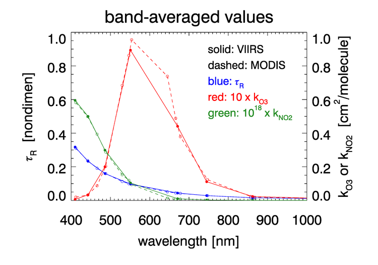
As was seen in for transmittance in Figs. 2 and 3, the absorption cross sections for gases like and, especially, can vary with wavelength on a nanometer scale. To fully resolve the effects of such wavelength dependence on sensor signals, radiative transfer calculations would require computationally intensive “line-by-line” calculations followed by integration over the sensor bands. To avoid that computational expense, band-averaged values of the Rayleigh optical depth and absorption cross sections and are computed for each sensor and tabulated. Radiative transfer calculations then use the band-averaged values with just one radiative transfer calculation done for each sensor band. These band-averaged values depend on the sensor even for the same nominal wavelength band (e.g, the 412 nm blue band) because of different band widths about the nominal center wavelength and different sensor response functions within a band. Figure 4 shows example band-averaged values for the VIIRS and MODIS Aqua sensors.
Absorption by
Nitrogen dioxide occurs both in the stratosphere and near the Earth’s surface. in the lower atmosphere is generated primarily by human activities (automobiles, industry, fires), and the highest concentrations are near the earth’s surface in industrial areas. Numerical simulations show that failure to correct for absorption by can give errors of approximately 1% in TOA radiances at blue wavelengths, which result in errors in retrieved water-leaving radiances (Ahmad et al. (2007)).
The geometric air mass factor of Eq. (1) and a simple atmospheric transmittance function like that of Eq. 2) are valid for ozone absorption corrections because scattering by ozone in the upper atmosphere is negligible. However, such functions may be not adequate for correction calculations because of multiple scattering in the dense lower atmosphere. Further guidance for the form of the correction comes from the observation that the water-leaving radiance sees all in the atmosphere, so the total concentration must be used to correct for absorption. However, the upwelling atmospheric path radiance , which is generated throughout the atmosphere, is not strongly influenced by the absorbing gas very near the surface. Extremely accurate numerical simulations show that in that case, , the concentration between an altitude of 200 m and the TOA, can be used as a satisfactory measure of concentration. This result leads to different corrections for the measured TOA path radiance and for the water-leaving radiance.
Let be the uncorrected, observed (measured) TOA reflectance, and let be the TOA reflectance corrected for absorption effects. Comparison of numerical simulations and analytical approximations justifies a correction of the form
where is the concentration between an altitude of 200 m and the TOA. This simple formula gives values that are within 0.15% of the values obtained by exact numerical simulations that account for the total column concentration and multiple scattering.
The correction for water-leaving radiance proceeds as follows. The reflectances can be written as (Ahmad et al. (2007), Eqs. 1 and 7)
(omitting the arguments for wavelength, azimuthal angle, and wind speed). Here is the diffuse transmission along the viewing direction from the sea surface to the sensor, is the diffuse transmission of downwelling solar irradiance, and is the water-leaving reflectance at the sea surface. Consider now only the path and water-leaving terms, and omit the directional arguments for brevity. Then multiplying this equation by the exponential correction factor for the observed TOA reflectance gives
Numerical simulations show that both the path reflectance and the diffuse transmission term are accurate to within 0.2% with this correction. However, the error in the water-leaving factor, is in error by 0.5 to 1.5%, which is unacceptably large. The reason for the greater error in this term is that it depends on the downwelling irradiance, which passes through the entire atmosphere and thus sees the total concentration , not just the reduced concentration that is adequate for correction of the TOA path term. However, the error in this term also decreases to if is replaced by . This error can be reduced still further by the following empirical procedure.
For bands where absorption is significant (e.g., at 412 or 443 nm), the atmospheric correction is determined as always (without correction) using the NIR bands. However, rather than subtract these terms from the corrected TOA reflectance, the atmospheric correction terms (including the Rayleigh reflectance) are reduced for absorption by applying a factor of . The computed path reflectance for is then subtracted from the observed TOA reflectance to obtain , which is the TOA value for water-leaving reflectance in the presence of . The -corrected value of the water-leaving reflectance is then obtained by multiplying this by , which gives
Note that is the -corrected transmission term, and is the desired -corrected water-leaving reflectance. This equation is then solved to obtain :
| (4) |
Note that the exponentials are increasing the magnitude of the water-leaving radiance compared to the no- case, which accounts for the loss due to absorption along the paths of the Sun’s direct beam and the viewing direction. The term for the Sun’s direct beam uses the full column concentration , whereas the viewing-path term uses the reduced concentration . This is an artifice that brings the analytical correction of Eq. (4) into close agreement with the exact numerical calculations. The absorption cross section is a function of wavelength. Computations are done for at 18 deg C, and then a temperature correction is made. (Ahmad’s Table 1 gives the band-averaged absorption cross sections for SeaWiFS and MODIS bands, which are called in that table. This is same quantity as in his Eq. (4) and in the equations of this chapter.)
 See comments posted for this page and leave your own.