The Atmospheric Correction Problem

An instrument viewing the ocean from a satellite or aircraft measures upwelling radiances that include contributions by the atmosphere, the water surface, and the water column. The atmospheric contribution $L_a$ comes from solar radiance that is scattered one or more times by atmospheric gases and aerosols into the direction of the sensor. The surface-reflected radiance (sun and sky glint) $L_r$ is downwelling solar radiance that is reflected toward the sensor by the water surface. The water-leaving radiance $L_w$ comes from light that is transmitted through the surface into the ocean, $L_t$, where it is changed by the absorbing and scattering components in the water, and is then scattered into an upward direction, $L_u$, and eventually leaves the sea surface in the sensor direction. Figure 1 shows this conceptually.

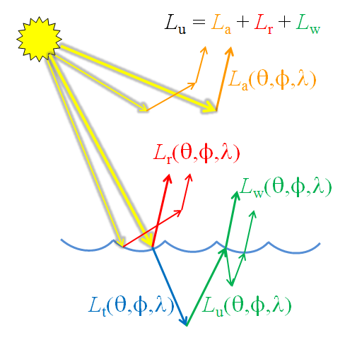
Radiance reflected by the sea surface contains information about the wave state of the surface, which may be of interest in itself or which, for example, may be useful for detection of surface oil slicks. Radiance scattered by the atmosphere along the path between the sea surface and the sensor contains information about atmospheric aerosols and other atmospheric parameters. However, only the water-leaving radiance carries information about the water column (and, in optically shallow water, about the sea bottom). A sensor looking downward measures the total radiance $L_u=L_a+L_r+L_w$ and cannot separate the various contributions to the total. Atmospheric correction refers to the process of removing the contributions by surface glint and atmospheric scattering from the measured total to obtain the water-leaving radiance.

[The term “atmospheric correction” offends some in the atmospheric optics community who rightly say that the atmosphere does not need correcting because it has not done anything wrong. They prefer to call the process “atmospheric compensation.” They make a valid point, but “atmospheric correction” is commonly used by those doing ocean color remote sensing, so that is what is used here.]

This page uses numerical atmosphere-ocean radiative transfer simulations to show examples of the nature and magnitude of the atmospheric correction problem. These figures were generated by a coupled MODTRAN-HydroLight radiative transfer code. The MODTRAN atmospheric code was used to propagate sunlight from the top of the atmosphere to the sea surface. The atmospheric radiance incident onto the sea surface was then used to initialize the HydroLight in-water code. HydroLight transmitted the radiance through the sea surface, computed its interaction with the water constituents, and eventually returned the water-leaving radiance back to MODTRAN. MODTRAN then propagated the water-leaving radiance, plus the glint radiance and atmospheric path radiance, to the sensor. Both of these codes are for unpolarized radiance calculations. The HydroLight-MODTRAN code can separate the Rayleigh vs. [aerosol + aerosol-Rayleigh] contributions, but cannot separate the pure aerosol from the aerosol-Rayleigh contributions. Likewise, it does not normally separate Sun glint and sky glint contributions, although that separation can be effected with some extra effort. The partitioning of atmospheric radiance contributions in the model simulations is thus not exactly the same as is done operationally, but the model simulations can still illustrate the various contributions to the TOA radiance.

Figure 2 shows examples of at-sensor total radiances $L_u$ for different sensor altitudes. The inputs to MODTRAN were for

• cloudless mid-latitude summer atmosphere
• marine aerosols
• relative humidity of 76% at sea level
• solar zenith angle of 50 deg
• surface wind speed of $6m{s}^{-1}$
• nadir-viewing sensor

These atmospheric conditions gave excellent remote-sensing conditions with a horizontal visibility of 63 km at sea level. The HydroLight inputs were for

• homogeneous water
• Case 1 water with a chlorophyll concentration of $1mg{m}^{-3}$
• infinitely deep water

The runs were from 300 to 1000 nm with 10 nm bandwidths. The sun and viewing geometry gives almost no sun glint radiance. However, there is always surface-reflected sky radiance, which shows up in the surface (zero altitude) spectrum (black curve) as non-zero $L_u$ radiance beyond 750 nm, where the water-leaving radiance is very close to zero. The differences in these curves are due solely to atmospheric contributions along the different path lengths from the sea surface to the sensor because all other conditions were the same for each curve. This figure shows that there is a noticeable atmospheric contribution to the total radiance even for sensors just a few hundred meters above the surface in very clear atmospheres. Airborne sensors typically fly at altitudes from 3,000 to 10,000 m, and even at lower altitudes the atmospheric contribution is greater than the water-leaving radiance. At 30,000 m, a sensor is effectively above the top of the atmosphere (TOA) and atmospheric path radiance is typically 90-95% of the total.

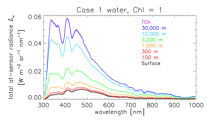
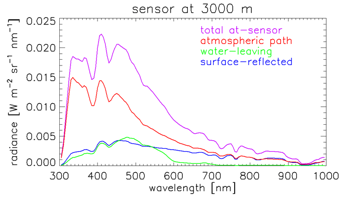
Figure 3 shows the Fig. 2 at-sensor radiance at 3,000 m partitioned into the contributions by water-leaving, surface-reflected, and atmospheric path radiances; the individual contributions can be separated in the numerical models. This altitude is typical for aircraft acquiring high spatial resolution hyperspectral imagery.

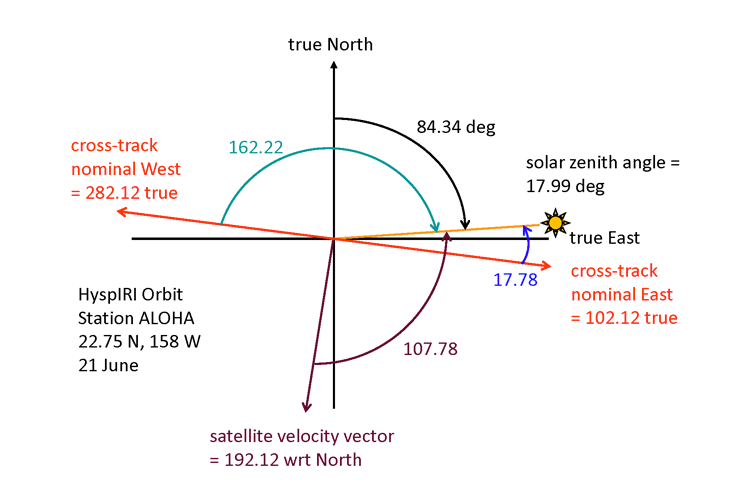
The atmospheric correction problem becomes even more intimidating when effects of sun and sensor viewing directions, atmospheric conditions, and surface wave state are considered. The following figures show a few examples of simulations performed in support of the design of the proposed NASA HyspIRI (Hyperspectral InfraRed Imager) mission. That sensor will measure radiances at the top of the atmosphere at 10 nm resolution from 380 to 2500 nm with 60 m ground resolution. The HyspIRI orbital characteristics were used to obtain the Sun zenith and azimuthal angles at the time the sensor would fly over a point at (latitude, longitude) = (28.75 N, 158.00 W) on June 21. This point is north of the island of Oahu in Hawaii and is known as Station ALOHA (A Long-term Oligotrophic Habitat Assessment). Figure 4 shows the relevant angles needed for the simulation.

The simulations shown below all have a chlorophyll value of $0.05mg{m}^{-3}$ characteristic of the very clear Case 1 ocean water near the Hawaiian Islands. The atmospheric conditions are for either a very clear tropical atmosphere (horizontal visibility of 100 km at sea level) or one with considerable haze (horizontal visibility of 10 km). The wind speed was 0 (a level sea surface) or $10m{s}^{-1}$. The sensor viewing direction was 30 deg east of nadir, nadir, or 30 deg west of nadir. The sun zenith angle was 18 deg, which corresponds to the time of the satellite overpass on 21 June at Station Aloha, near Hawaii.

A simulation was done for the following environmental conditions:

• The water was homogeneous and infinitely deep.
• The water IOPs were simulated using a chlorophyll concentration of $Chl=0.05mg{m}^{-3}$ in the new Case 1 IOP model in HydroLight.
• The Sun zenith angle was ${𝜃}_{Sun}=17.99deg$ and the Sun’s azimuthal angle was east of the nadir point at 84.34 deg from true north.
• The off-nadir viewing angle was ${𝜃}_v=30deg$, ${\varphi }_v=281.12deg$, which is at right angles to the satellite’s orbital direction and looking to the west side of the orbit, away from the Sun’s direction.
• The atmospheric conditions (temperature profile, water vapor, ozone, etc.) were typical of a tropical marine atmosphere (defined via MODTRAN’s “Tropical Atmosphere” option). The sky conditions were clear. The aerosols were for an open-ocean marine atmosphere.
• The wind speed was $10m{s}^{-1}$.
• The wavelength resolution was 10 nm from 350 to 1500 nm.

Figure 5 shows various radiances and irradiances obtained from this simulation. The solid curves are values at the TOA, and the dotted curves are the corresponding quantities just above the sea surface. The $E_d$ TOA curve (the solid purple line) is the extraterrestrial solar irradiance (averaged over 10 nm bands) on a surface parallel to the mean sea surface. The dips in the curve below 700 nm are due to absorption by various elements in the Sun’s photosphere; these are Fraunhofer lines averaged over the 10 nm bands of this simulation. Above 700 nm, the Sun’s irradiance is close to a blackbody spectrum. The purple dotted line shows how much of the TOA solar irradiance reaches the sea surface. There are large dips in the TOA irradiance that reached the sea surface in the regions around 940 and 1130; these are due to absorption by water vapor, as are the smaller dips near 720 and 820 nm. The large opaque region between 1350 and 1450 nm is due to water vapor and carbon dioxide. The dip at 760 nm is due to absorption by atmospheric oxygen. These absorption features of the Earth’s atmosphere will affect any radiation passing through the atmosphere.

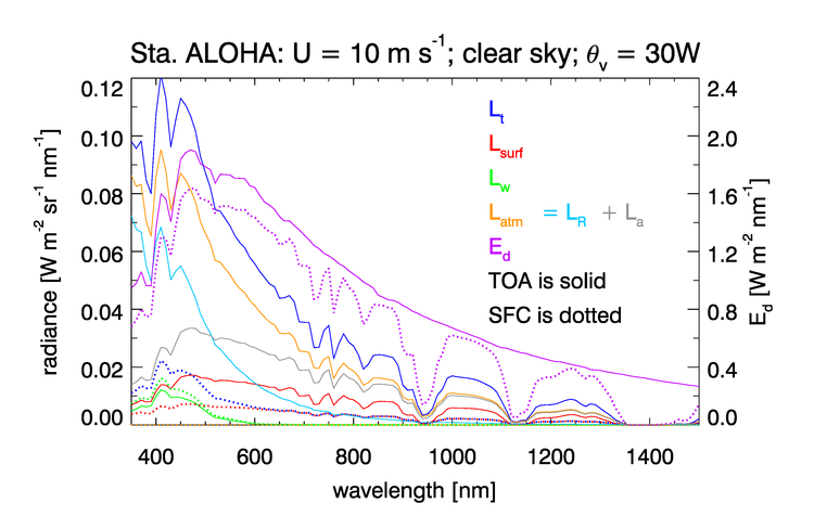
The solid blue line shows the TOA radiance $L_t$ that would be measured by a satellite looking in the direction 30 deg West of the nadir point. The orange curve shows how much of the total is atmospheric path radiance, $L_{atm}$. The aqua and gray curves respectively show how much of the path radiance is due to Rayleigh scattering by atmospheric gases and by aerosols (including aerosol-gas interactions). The green curves in Fig. 5 show that the water-leaving radiance at the TOA (the solid curve) is less than the water-leaving radiance just above the sea surface (the dotted curve). This makes intuitive sense, because part of the water-leaving radiance would be lost to atmospheric absorption or scattering into other directions before that radiance reaches the TOA.

The red curves show the total radiances due to surface reflectance, i.e., the sum of the background sky reflectance and the direct Sun glint. However, the red curves show that the surface-reflectance contribution is greater at the TOA than at the surface. This seems counterintuitive and requires explanation. Figure 6 gives a more detailed view of the contributions to the TOA radiance. In this figure, the arrow labeled $L_g$ represents Sun glint due to the occasional wave facet that is tilted in just the right direction to create glint that is seen by the sensor. The arrow labeled $L_{gs}$ represents the very bright glint in the Sun’s specular direction; the sensor is looking in the direction away from the Sun’s azimuthal direction in order to avoid viewing this specular glint. However, the specular glint gives a strong reflected radiance, some of which is being scattered by the atmosphere into the sensor viewing direction; this is illustrated by the $L_{gs2}$ arrow in Fig. 6. The surface contribution in Fig. 5 is the sum of the $L_{sky}$, $L_g$, and $L_{gs2}$ contributions. If the ocean is viewed from just above the sea surface (the red dotted line in Fig. 5), the surface-reflected radiance comes only from reflected sky radiance $L_{sky}$ and a small amount of direct Sun glint $L_g$ from wave facets that are tilted in just the right way to reflect the Sun’s direct beam into the direction of the sensor. (This direct Sun glint $L_g$ is minimal because of the choice of viewing direction.) These surface-reflected sky and Sun radiances decrease between the surface and the TOA, just as does the water-leaving radiance. However, the total TOA radiance that arises from sea surface reflectance, as partitioned in the simulation, comes from the sum of the surface reflectance in the viewing direction (decreasing with altitude) and the contribution by atmospheric scattering of specular Sun glint into the viewing direction ($L_{gs2}$, increasing with altitude). The specular radiance $L_{gs2}$ is large in magnitude, so the atmospheric scattering of this radiance into the viewing direction can be significant. If the present simulation is run with a level sea surface, for which there is no $L_g$ Sun glint into the sensor direction, this behavior is still present and, indeed, is even somewhat greater in magnitude. (To fully isolate the effect of specular Sun glint being atmospherically scattered into the sensor, a special run was made in which any ray from the Sun’s unscattered beam that was reflected by the sea surface was killed. That is, all Sun glint was forced to be zero. Only rays from the background sky that were reflected by the sea surface were allowed to contribute to the TOA surface-reflected radiance. In that case, the surface-reflected radiance behaves the same as the water-leaving radiance: less sky glint reaches the TOA than leaves the sea surface.)

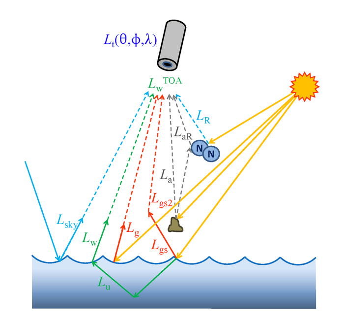
Figure 7 shows the fractional contributions by these various processes to the total TOA radiance $L_t$. For this particular case, the water-leaving radiance is at most 10% of the total TOA radiance. The atmospheric path radiance contributes 70 to 90% of $L_t$, with the rest coming from surface glint. Below 500 nm, Rayleigh scattering by atmospheric gases is the largest contributor to the TOA radiance. This is also true in the band from 1350 to 1400 nm, where the atmosphere is essentially opaque, because the aerosols are located mostly near the sea surface. Aerosols are the greatest contributor between 500 and 1350 nm.

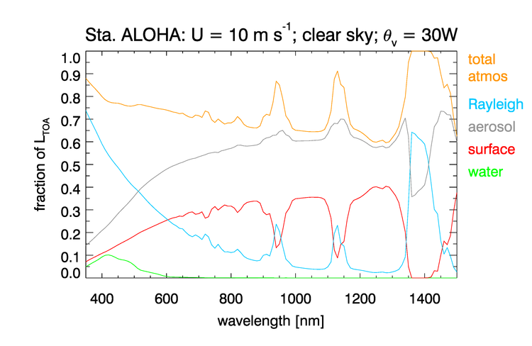
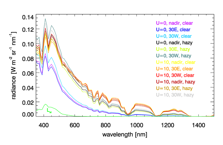
Figure 8 shows the $L_t$ of Fig. 5, plus the corresponding $L_t$ radiances for wind speeds of 0 and $10m{s}^{-1}$, clear and hazy atmospheric conditions, and viewing directions of 0 (nadir) and 30 deg East or West of the flight direction. Each of these 12 much-different TOA radiances has essentially the same water-leaving radiance $L_w$, which is shown in green.

The atmospheric correction problem can be visually summarized as follows: Given any of these TOA radiance spectra seen in Fig. 7 and the geometry (Sun location and viewing direction), recover the water-leaving radiance spectrum $L_w$. This is clearly a difficult problem because the needed atmospheric conditions (aerosol type and concentration in particular) are not obtained as part of the $L_t$ measurement.

Atmospheric correction is the central problem of ocean color remote sensing. However, the problem is not intractable—if it were, we could not do ocean color remote sensing! There are many inversion algorithms that can retrieve ocean properties such as chlorophyll, mineral, or CDOM concentrations, or bottom depth and reflectance, IF an accurate water-leaving radiance (or, usually, its equivalent reflectance, to be developed on then