Page updated:
March 22, 2021
Author: Curtis Mobley
View PDF
Autocovariance Functions: Sampling
This page shows exactly how the calculations underlying the first, third, and fourth figures of the previous page were performed. The devil is in the details, and these details are seldom (if ever!) discussed in the literature. Consider the case of , which will allow individual points to be plotted. Of course, with so few sample points, the variance spectrum is not adequately sampled and the resulting sea surface is unphysical because it has far too little variance. However, the algorithms are the same for any value of .
Consider first the generation of the random sea surface with points. As discussed previously, the two-sided spectrum must be sampled at exactly spatial frequencies. The green dots in Fig. 1(b) show these points for the case of . The frequency values, written in math order, are
| (1) |
which for the choice of and gives
| (2) |
where . Here braces denote a set of frequencies labeled by values, and brackets denote an array of frequency values as shown. Note that the sampled frequencies are symmetric about , except for one “extra” point at index or frequency . This value is the Nyquist frequency, which in IDL is stored as the last element of the frequency array in math order. Sampling the spectrum at exactly this pattern of frequencies guarantees that the spectral amplitudes generated from them are Hermitian, which in turn guarantees that the generated sea surface is real. The red dots in Panel (c) of the figure show the 8 surface elevations generated for a particular sequence of random numbers. The values are at to for to . Fourier-generated surfaces are inherently periodic, so that .
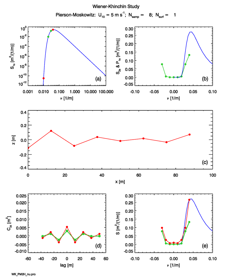
Now take the inverse DFT of the discrete spectrum given by the green dots in Panel (b). The result is the autocovariance values shown by the green dots in Panel (d). It is important to note that these lag values follow the same pattern (in math order) as the frequencies:
| (3) |
where now . The lags are symmetric about , except for one “extra” point at . This is analogous the one extra value in the frequency spectrum at the Nyquist frequency. Taking the forward DFT of these 8 autocovariance values as in Eqs. (10) and (11) on the Autocorrelation Functions: Theory page gives the green points plotted in Panel (e). These values are of course exactly the 8 points of the original spectrum, as shown by the green dots in Panel (b). This is just a check on the correct implementation of the round-trip calculation of inverse and forward Fourier transforms.
Now suppose that we wish to compute the autocovariance of the surface elevations, and from that obtain an estimate of the variance spectrum via the Wiener-Khinchin theorem. This provides a more stringent test of the calculations because of the intermediate sea surface in between the variance spectrum and the autocovariance. The crucial observation is that when calling the IDL autocovariance routine A_CORRLELATE, that routine must be given an array of the requested lag indices (lags in units of ) as seen in Eq. (3). Thus for an array of surfaces,
| (4) |
an array of lags
| (5) |
must be defined. The call to the IDL routine is then
| (6) |
The IDL routine then returns an array of autocovariances at the lags shown in Eq. (3). These values are shown by the red dots in Fig. 1(d). This array returned by A_CORRLELATE has the same math order as the array. This array must next be shifted into the FFT order via the IDL shift function:
| (7) |
This array can now be given to the IDL FFT routine:
| (8) |
The resulting array is a complex 8-element array. The real part of is , with the frequencies in FFT order. The imaginary part is zero (to within a bit of roundoff error; values are typically less than ). This array is shifted back to math order and divided by to get the array plotted as the red dots in Panel (e) of the figure:
| (9) |
It is always informative to take an “information count” of such operations. We started with a two-sided spectrum of 8 values. It is true that in the present time-independent simulations (except for the 0 and Nyquist frequencies, which are always special cases). However, this symmetry need not hold in general (and indeed is not the case when generating waves that propagate downwind, as explained previously). Thus these spectrum values represent 8 independent “pieces” of information in the form of 8 real numbers.
The 8 elevations of the sea surface are likewise 8 independent pieces of information.
Finally, the 8 covariances also comprise 8 pieces of information. Similarly to the variance spectrum, there is symmetry about the 0 lag, except for the value at the largest positive lag. However, again, the fact that represents two pieces of information: the value of and the fact that has the same value.
Thus the sampled variance spectrum , the generated surface , and the surface autocovariance all contain the same amount of information, namely 8 real numbers. The various Fourier transforms and autocorrelation function show how to convert the information from one form to another.
Idle Speculations
It is certainly possible to sample in different ways. For example, surface correlations can be computed for all lags from to , which gives total values. You can then take the FFT of that covariance and get a spectrum with values. However, I can guarantee you from two weeks of misery that the spectrum so obtained does not agree with the original spectrum. The extra points added by taking a greater range of correlations are in some way not independent of or consistent with the independent pieces of information tallied above. That is to say, the sea surface contains only pieces of information, and you cannot create more information simply by computing the autocovariance at more lag values. I vaguely remember reading somewhere that you should not compute autocovariances for lags greater than one-half of the data range. Note that the lag indices used above run from values of to , which indeed correspond to the to data range. I suspect, but have never seen stated, that there is something going on here that is analogous to sampling at greater than the Nyquist frequency—You can do it, but it messes up the results in ways that are not immediately obvious.
Another possible way to compute the autocovariance for a given sea surface is to compute only for 0 and positive lags out to a maximum possible lag of . This would again give independent numbers. Autocovariances are real and even functions of the lag (symmetric about ), which means that their Fourier transforms are also real and even. Since , a Fourier transform can be written as the sum of a cosine transform plus times a sine transform: . Here the cosine transform is defined as in Eq. (1) of the Fourier Transforms page except that is replaced by ; the sine transfrom is defined in the same way but with replacing . For an even function, the sine components in the Fourier transform will all be zero. Thus it seems that the Wiener-Khinchin theorem could be written as . An example of this was seen above in the analytical computation of the Horoshenkov variance spectrum. However, there are four different algorithms for implementing the discrete cosine transform (DCT), which differ by how the discrete, finite- sequence of points is assumed to be extended outside the domain for which is known. It seems that the present case of , which is symmetric about , corresponds to the “Type I” DCT discussed at https://en.wikipedia.org/wiki/Discrete_cosine_transform or the “” extension seen in Fig. 2(a) of Makhoul (1980). The four different formulations of the DCT can be computed in four different ways by use of FFTs. Thus the use of a DCT for the discrete Wiener-Khinchin theorem opens a new can of worms. In any case, there is little or no penalty to be paid for sticking with a Fourier transform evaluated by an FFT routine in order to evaluate the DFTs as needed here. As a matter of practical necessity, the internal consistency of the spectra, surfaces, and autocovariances seen in the preceding figures (and to be seen below) indicate that the sampling scheme described above is correct, even it there may be equivalent ones.
Lessons Learned
The preceding simulations illustrated the Wiener-Khinchin theorem starting with a variance spectrum (the Pierson-Moskowitz spectrum) and arriving at an autocovariance in two ways. The first way was to construct the corresponding two-sided spectrum and then take the inverse Fourier transform to obtain the theoretical, noise-free via the Wiener-Khinchin theorem. The second way was to use to generate a large number of random sea surfaces. The autocovariance of each random surface was computed by Eq. (3) of the Autocovariance Functions: Theory, and then the ensemble-average autocovariance was computed as the average of the individual autocovariances.
It is important to note that the size of the spatial region and the number of sample points must be chosen with care. As a rule, must be large enough to cover several wavelengths of the longest wave that contains a significant amount of the total variance. must be large enough that the sampled points on the variance spectrum then reach far enough into the high-frequency end of the spectrum to cover the entire part of the spectrum that contributes a significant amount to the total variance. To see the effects of inadequate sampling, suppose we are concerned only with the short gravity and capillary waves, which are optically the most important because they have the highest slopes. If we are interested only in waves of wavelength down to , it might then seem reasonable to let and , which give . The shortest resolvable wavelength is then . Figure 2 shows an example surface and other quantities for this case.
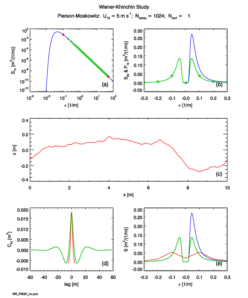
However, now and the spectrum is sampled only at widely spaced points (the green dots in Panel (b)) that largely miss the peak of the variance spectrum. Consequently, the generated surface has too little variance compared to the real sea surface described by this spectrum. Also, the sample autocovariance function, shown by the red curve in Panel (d), computes the autocovariances only for lags up to . This lag range does not capture the full autocovariance features of the real surface, for which the autocovariance is non-zero out to lags of , as shown by the green curve in Panel (d). The spectrum estimated from the sample autocovariance (the red curve in Panel (e)) does reproduce the sampled spectrum (the green dots in Panel (b)), but this spectrum is not representative of the real sea surface.
Picking , as in the previous simulations, seems adequate for a wind speed of . This can be seen from the leftmost red point in Panel (a) of the previous plots, which is to the left of the spectrum maximum. However, then gives , and the last sampled point corresponds to a shortest resolvable wavelength of . If that is not adequate resolution for the problem at hand, there are two options. One option is to increase , which costs more computer time to evaluate the FFTs. The other option is to adjust the spectrum in some way to account for the missing variance while keeping relatively small. One technique for doing such a spectrum adjustment is described on the Numerical Resolution page.
Increasing by a factor of 8 to then gives , which might be adequate for the problem at hand. The time for an FFT is proportional to , so that increase in comes at a factor-of-ten increase in run time, which can be prohibitive if many surfaces must be generated. The other option is to account for the unsampled variance in some other way. One technique for doing that is to adjust the spectrum to account for the missing variance while keeping relatively small. One technique for doing this is described on the Numerical Resolution page.
These results can be summarized as follows:
- The size of the spatial domain, , must be large enough to cover at least several wavelengths of the wave of maximum variance. The value of sets the fundamental frequency , which equals the frequency interval .
- For the given fundamental frequency , the number of spatial samples, , must be large enough that the highest (Nyquist) frequency, covers the domain of the variance spectrum for which the variance is non-negligible. This highest sampled frequency must also cover the highest frequency (shortest wavelength) needed for the problem at hand. The minimum resolvable wavelength is .
Of course, the need for large and large comes as the cost of increased computer time. Experimentation is necessary to determine what values are required for a particular physical situation.
 See comments posted for this page and leave your own.