Ray Tracing

The previous page showed how to determine ray path lengths and scattering angles using the beam attenuation $c$, the scattering phase function $\tilde{\beta }$, and a uniform $U\left[0,1\right]$ random number generator. This page shows how to combine those two processes to create random ray paths through an absorbing and scattering medium.

Ray Tracing

There is more than one way to simulate ray paths, and each will give the same answer. However, some techniques can be numerically much more efficient than others. Indeed, a reasonable approach to developing a Monte Carlo algorithm for a particular problem is to

1.

first figure out how to numerically simulate a process as it occurs in nature, and

2.

then figure out how to simulate another, perhaps artificial, process that will give the same answer as the “natural” process, but with less computational time.

This page illustrates this two-step development process.

Consider first how rays propagate through a medium. Loosely speaking, a ray travels until it interacts with a particle, e.g. a molecule of water or chlorophyll. It is then either absorbed by the particle and disappears, or it is scattered into a new direction and continues on its way until in interacts with another particle.

Recall the albedo of single scattering, ${\omega }_o=b∕c$. If there is no absorption, $b=c$ and ${\omega }_o=1$. If there is no scattering, $b=0$ and ${\omega }_o=0$. ${\omega }_o=b∕c$ thus can be interpreted as the probability of ray survival in any particular interaction. When a ray encounters a particle, we can randomly decide if the ray is to be absorbed or scattered as follows:

1.

Draw a random number $𝔯$ from a $U\left[0,1\right]$ distribution.

2.

Compare $𝔯$ with ${\omega }_o$.

• If $𝔯\le {\omega }_o$, then the ray is scattered.
• If $𝔯>{\omega }_o$, then the ray is absorbed.

If the ray is absorbed, tracing stops and a new ray is emitted from the source and tracing begins anew. If the ray is scattered, two new $U\left[0,1\right]$ random numbers are drawn and used to determine new polar and azimuthal scattering directions $\psi$ and $\chi$ as shown on the previous page. Another random number is used along with $c$ to determine the distance traveled before another interaction.

Figure 1 illustrates this process for two rays, which also introduces the geometry to be used in numerical simulations below. A source emits a collimated beam of rays, which are then recorded by an annular, ring, or ”bullseye” detector some distance away. The red ray is emitted by the source, undergoes one scattering, and is then absorbed by a particle. The green ray is emitted, undergoes two scatterings, and is recorded by a detector.

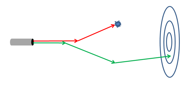
This process mimics what happens in nature. Call this ”Type 1” ray tracing (there are no standard names for ways of tracing rays). Note that all of the computations used to trace the absorbed ray are wasted because the ray never reached the detector. Nature can afford to trace innumerable rays and waste some by absorption, but that is not advisable for most numerical simulations. We therefore seek other ways to trace rays.

The previous page showed that the mean free path or average distance between interactions with the medium is $1∕c$. These interactions can result in either absorption or scattering of the ray, as just described. Rather than tracing one ray at a time as nature does, consider a source emitting “bundles” of many rays (often called “photon packets” in the literature). Then view each interaction as having a fraction $1-{\omega }_o$ of the rays in the bundle being absorbed, and the remaining fraction ${\omega }_o$ being scattered, all in the same direction. Let the bundle be emitted with an initial weight of $w=1$, which can represent one unit of energy, power, or some number of rays. At each interaction, the current weight $w$ is multiplied by ${\omega }_o$ to account for the loss of energy or number of rays by absorption (that is, a fraction ${\omega }_o$ continues onward). The scattered bundle then carries a reduced weight. If the ray bundle reaches the target, the current weight $w$ is tallied. Another bundle is then emitted from the source and traced. This tracing process, which we’ll call ”Type 2,” is illustrated by the green ray track in Fig. 2. After two scatterings, as illustrated, the detected ray bundle has weight $w={\omega }_o^2$.

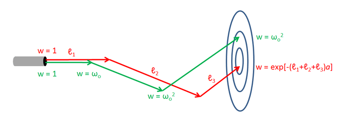
A third ray-tracing process can be envisioned. The mean distance traveled between scattering events is $1∕b$. We can thus use $1∕b$ and a random number to determine the distance between scattering interactions, and the initial weight of $w=1$ is not changed at each interaction because all rays in the bundle are viewed as being scattered. Then, if the ray bundle reaches the target, absorption is treated as a continuous process occurring along the entire ray path. Assuming homogeneous water, the final weight tallied is then $e^{\left(-\ell a\right)}$, where $\ell$ is the total path length in meters and $a$ is the absorption coefficient. The red track in Fig. 2 illustrates this ”Type 3” ray tracing. The red track shows a total path length of ${\ell }_1+{\ell }_2+{\ell }_3$, so the final weight is $e^{-\left[\left({\ell }_1+{\ell }_2+{\ell }_3\right)a\right]}$.

The two tracks in Fig. 2 are drawn as though each track were generated by exactly the same sequence of random numbers. Because $1∕b>1∕c$, the individual Type 3 ray paths will be greater than the Type 2 paths. The scattering angles are the same. Thus these two tracing types clearly lead to different results, ray bundle by ray bundle. However, numerical simulation of many ray bundles shows all three of these ray tracing types yields the same distribution of energy at the detector.

To summarize, the three types of ray tracing considered here are

Type 1:

Individual rays are tracked, and rays can be absorbed.

Type 2:

Ray bundles are tracked, with a bundle weight being multipled by ${\omega }_o$ at each interaction.

Type 3:

Ray bundles are tracked, with track lengths determined by the mean free path for scattering, no weighting at scattering events, and absorption treated as a continuous process based on total path length.

Numerical Comparison of Tracking Types

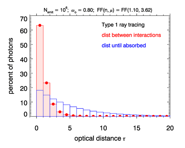
To illustrate the results obtained for different ways of tracking rays, a Monte Carlo code was written to simulate the energy received by an annular target as illustrated in Figs. 1 and 2. For the simulations shown here, the IOPs were defined by $a=0.2m^{-1}$, $b=0.8m^{-1}$, and a Fournier-Forand phase function with parameter values $\left(n,\mu \right)$ = (index of refraction, slope of Junge distribution) chosen to give a good fit to the Petzold average particle phase function. Thus ${\omega }_o=0.8$, and optical distance $\tau$ is numerically the same as geometrical distance $\ell$ in meters. A run was made with $10^6$ rays being sent from the source and using Type 1 ray tracing. rays were traced until they were absorbed. Figure 3 shows some of the resulting statistics.

The red histogram shows the percent of rays that traveled an optical distance ${\tau }_1\le \tau \le {\tau }_2$ between interactions, for a bin size of ${\tau }_2-{\tau }_1=1$. The theoretically expected fraction of rays traveling an optical distance between ${\tau }_1$ and ${\tau }_2$ between interactions is

The red dots in the figure are the expected values given by this formula. The shortest ray path length between interactions was $\tau =1.192\times 10^{-7}$ and the longest was 16.69. The blue histogram shows the distribution of total distances traveled until the rays were absorbed. Thus the value for the first bar shows that about 18% of the rays were absorbed after going a total optical distance between 0 and 1. Note that this distance can represent more than one interaction, i.e., a ray being scattered one or more times before being absorbed. Both the red and the blue histograms sum to 100%. As shown on the previous page, the mean distance traveled between interactions is $\tau =1$, or $1∕c$ in meters. For this particular simulation the actual average was $\tau =0.9974$ (or 0.9974 m for these IOPs). The small difference is statistical noise resulting from the finite sample size of the numerical simulation. Likewise, the average distance traveled until the rays are absorbed is $1∕a$. For the present case of $a=0.2m^{-1}$ this gives 5 m. The average for this simulation was 4.9949 m. Since $c=1m^{-1}$ for this simulation, another way to view this is that the rays were on average scattered four times before being absorbed on the fifth interaction.

We next compare results for the three different ways of tracking rays. Because oceanic phase functions scatter much more light at small scattering angles than at large angles, most rays that are scattered just a few times will hit the detector near its center. To even out the numbers of rays (or power) detected by each ring, an annular target was defined with a logarithmic spacing for the radii of the detector rings. A logarithmic spacing is often used in instruments so that each detector ring receives roughly equal amounts of power, which reduces the dynamic range needed for the instrument design. The detector simulated here had $N_{rings}=10$ rings with the smallest ring radius being $r_{min}=0.1$ and the largest being $r_{max}=10$. This detector is placed in a target plane some distance $z_T$ from the source and centered on the optical axis of the source, as shown in Figs. 1 and 2. The rays crossing the detector plane at some distance $r$ from the detector center are tallied in bins as follows:

Bin $0$:

Unscattered rays that hit the detector at $r=0$.

Bin $1$:

Scattered rays that hit the target plane inside the first detector ring, i.e. at $0<r<r_{min}$.

Bins $2,...,N_{rings}+1$:

rays that hit detector rings 1 to $N_{rings}$.

Bin $N_{rings}+2$:

rays that hit the detector plane outside the outer ring, i.e. at $r>r_{max}$.

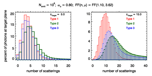
Simulations were made with $N_{emit}=10^6$ rays (for Type 1) or ray bundles (Types 2 and 3) emitted from the collimated source. Figure 4 shows the distribution of rays or bundles received anywhere in the detector plane as a function of the number of scatterings, for the three types of tracing and for target plane distances of $z_T=5$ and 15. The left panel shows that for $z_T=5$ one or two percent of rays (depending on the tracing type) reach the target plane without being scattered. Most rays are scattered 3 or 4 times, and very few rays are scattered more than 10 times. The right panel shows that for $z_T=15$, almost no rays reach the target plane unscattered, and most undergo 5 to 25 scatterings, with a peak around 10 or 15, depending on the way the rays are traced. For Type 1 ray tracing, almost no rays are scattered more than 30 times. Note that the probablity of surviving 30 scatterings is ${\omega }_o^{30}=0.0012$. For tracing Types 2 and 3, which never have ray bundles absorbed, there are broad tails in the number of scatterings, although for Type 2 a bundle being scattered 40 times has an almost negligible weight of $w={\omega }_o^{40}=0.00013$.

The left panel of Fig. 5 shows the intersection points of the rays reaching a $\tau =10\times 10$ area of the target plane for the first $10^4$ emitted rays, tracing Type 1, and the target plane at $z_T=5$. Note that of the $10^4$ emitted rays, only 2973 reached the target plane (of which 2966 are in the area plotted). This is less than 30% of the rays making a contribution to the answer of how much power is detected; i.e., 70% of the calculations were wasted. The ray-intersection dots are color-coded to show the number of times each plotted point was scattered. The two black circles show off-axis angles of $30^{\circ }$ and $60^{\circ }$. Very few rays were scattered more than about $30^{\circ }$ off of the optical axis. The right-hand panel shows the distributions of the rays reaching the target plane by number of scatterings and total distance traveled. Every ray must of course travel a distance of at least $\tau =5$ before reaching the target plane, and most rays were scattered several times.

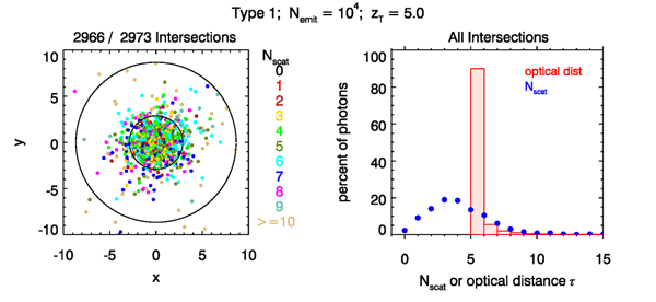
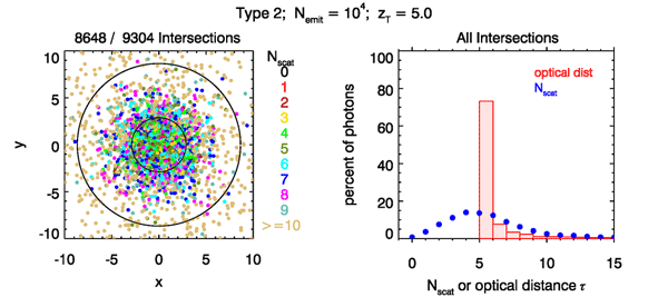
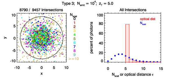
Figure 6 shows the same distributions for Type 2 scattering. Note than now 93% of the emitted ray bundles eventually intersect the target plane. Only 7% of the emitted rays were wasted. Those rays ended up being scattered into directions away from the target plane (either by backscattering or by multiple large-angle forward scatterings). Figure 7 shows the results for Type 3 tracing. The distributions are similar to those for Type 2, but with over 94% of the rays reaching the target plane.

Figures 8-10 show the corresponding results when the target plane is at $z_T=15$. Now, for Type 1 tracing, only 179 of $10^4$ emitted rays ever reached the target plane. Over 98% of the ray-tracing calculations were wasted! Note also that there is obvious statistical noise in the distributions of the right panel, due to the small number of rays used to computed the statistics. For Types 2 and 3 about 71% and 82%, respectively, of the emitted rays eventually reach the target plane. The statistical noise is now much smaller (but still noticeable) because of the larger number of ray bundles.

The total optical distance distributions for Types 2 and 3 show broad tails. In both cases, fewer than one fourth of the rays made it to the target plane after traveling a total distance of $\tau =15–16$. About 30% of the rays underwent 30 or more scatterings and traveled a distance of $\tau \ge 30$. These broad tails illustrate the phenomenon of pulse stretching in time-dependent problems. If we think of all $N_{emit}$ rays being emitted simultaneously, then the longer distances traveled correspond directly to later arrival times at the target. Pulse stretching is an important limiting factor in time-dependent applications such as lidar bathymetry or communications with high-frequency light pulses.

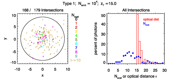
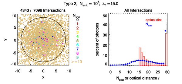
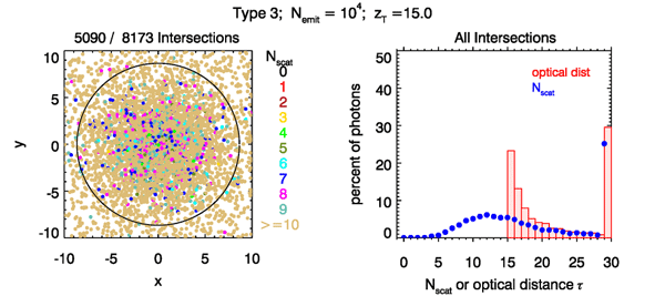
Figure 11 shows the distributions of numbers of rays at the target plane and the corresponding power (or energy) for the three tracing types and the detector at $z_T=5$. The left panel shows the distributions as a function of the detector ring radii, and the right panel is the same information as a function of the bin number defined above. Recall that the first abscissa point is unscattered rays, the second is scattered rays inside the first detector ring, and the last plotted point is for rays outside the last detector ring. The solid-line histogram represents the 10 detector rings for $r_{min}=0.1<r<r_{max}=10$.

There are several things to notice in this figure. First, the distributions of the numbers of rays (open circles) are different for the three tracing types. For Type 1, the distribution of the number of rays is the same as the power distribution because the rays all retain their initial weight of $w=1$. Thus power detected is simply the number of rays detected. For Types 2 and 3, more rays are detected, but each is weighted less to account for absorption along the way. Finally—and most importantly—the power distributions for these three tracing types are identical to within a small amount of statistical noise, which is not visible in these plots.

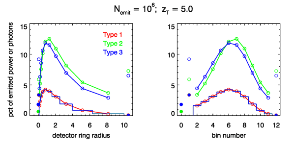
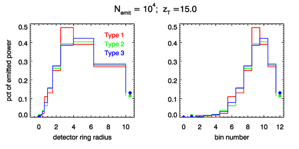
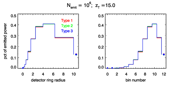
Figure 12 shows the power distributions for the detector at $z_T=15$ but only $N_{emit}=10^4$ rays emitted. There are obvious differences in the distributions for the three tracing types. However, if $N_{emit}=10^6$ rays are traced, as in Fig. 13 these differences almost disappear. This indicates that the three ways to trace rays all give identical predictions of the detected power, to within some amount of statistical noise, which can be reduced by tracing more rays.

However, the computation time required by the three tracing types can vary greatly. Recall from Fig. 5 that about 30% of the rays reached the target plane at $z_T=5$ for Type 1 tracing, but that over 90% reached the target plane for Types 2 and 3 (Figs. 6 and 7). Thus, if we require a certain number of detected rays to achieve some desired level of statistical noise, we would have to emit and trace over three times as many rays for Type 1 tracing (hence three times the computer time) as for Type 2 or 3. For the detector at $z_T=15$ and Type 1 tracing, fewer than 2% of the emitted rays reached the target plane (Fig. 8), whereas about 80% of the rays reached the target plane for Types 2 and 3 (Figs. 9 and 10). Getting the same number of rays on target would thus require emitting over 40 times as many rays (hence 40 times the computation time) for Type 1 as for Types 2 or 3.

We have now shown that several ways of tracing rays can be devised and that each gives the same distribution of power or energy at a detector some distance away from the source. However, an intelligent choice of the ray tracing algorithm can greatly reduce the needed computations. Moreover, the computation differences depend on the particular problem, e.g., on detector distance from the source as shown here (or on the IOPs, not shown here). However, we can do still more to reduce computation times, which leads us to the next topic of variance reduction techniques.