Page updated:
April 12, 2021
Author: Xiaodong Zhang
View PDF
Air Bubbles
Bubbles in the upper ocean are primarily generated by breaking waves (Lamarre and Melville (1991); Thorpe and Humphries (1980)). When wind speed exceeds , field observations have shown that a stratus layer of bubbles forms under the sea surface and persist as a result of continuous supply of bubbles by frequent wave breaking and the subsequent advection by turbulence (Crawford and Farmer (1987); Thorpe (1982); Thorpe (1986)). As wind subsides, bubbles that have been injected will evolve under the effects of buoyancy and gas diffusion, and merge into the background population on time scales of minutes to hours (Johnson (1986)). When wind speeds are lower than , few waves break (Thorpe (1982); Thorpe and Hall (1983)). In quiescent conditions, the presence of bubbles has also been detected (e.g. Medwin (1977); O’Hern et al. (1988)), and the sources of these bubbles have been attributed to the pre-existing cavitation nuclei (O’Hern (1987)), remnant of bubbles injected by breaking waves (Johnson (1986)), sediment outgasing (Mulhearn (1981)), phytoplankton photosynthesis (Waaland and Branton (1969)), or zooplankton respiration (Ling and Pao (1988)).
Once formed, bubbles are coated with surfactant material almost instantaneously and the accumulation of organic films onto their surfaces provides a stabilizing mechanism against surface tension pressure and gas diffusion (Fox and Herzfeld (1954); Yount (1979)). These stabilized bubbles, acting as cavitation nuclei, explain the tensile strength (Apfel (1972)) and cavitation pressure (Holl (1970)) observed for natural water with magnitudes that are much lower than theoretical predictions for pure water.
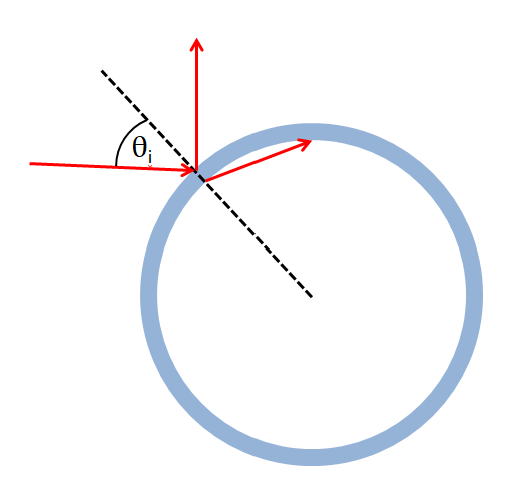
The first study of optical properties of an air bubble in water probably carried out by Davis (Davis (1955)), who used the geometric optics approximation to study the angular distribution of intensity of light scattered by an air bubble in water. Later, the most intensive studies of single bubble optics were undertaken by Marston and co-workers (Arnott and Marston (1988a); Arnott and Marston (1991); Arnott and Marston (1988b); Kingsbury and Marston (1981); Marston (1979); Marston et al. (1988); Marston and Kingsbury (1981); Marston et al., 1982)). They examined light scattering pattern near the critical angle (), Brewster angle (), and glory (). As shown in Fig. 1, a bubble (large compared to the wavelength of incident light) suspended in water can be regarded as a local water-to-air interface. When the incident angle is equal to or greater than (), the light experiences total reflectance with a scattering angle of or larger. Similarly when the incident angle is (), the parallel polarized light has a null reflectance according to Fresnel’s law, and the light at scattering angle of is entirely perpendicularly polarized. Analogous to the optical glory of a drop but with different mechanism, light scattered from bubbles in water manifests an enhancement in the backward direction ). The viewable enhancement is within a circle of radius of about .
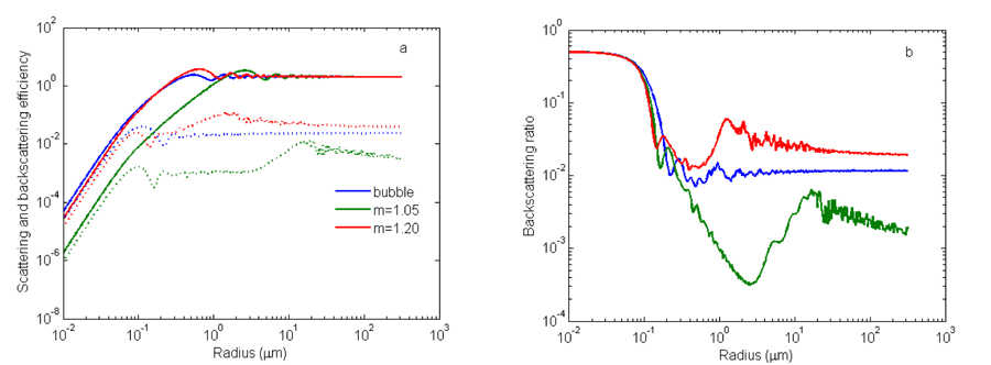
For rising bubbles, their shape will become oblate due to drag, which in turn depends on the bubble size, surfactant, and water kinematic viscosity. By observing the glory pattern exhibited by freely rising bubbles, Arnott and Marston (Arnott and Marston (1988b)) found that for bubbles with radius , the shape is sufficiently spherical for Mie theory to be valid. Also photographs show that bubbles with adsorbed monolayers of surface-active material remain spherical (Johnson and Cooke (1981)). For practical purpose, bubbles in the ocean are assume to be spherical and the errors introduced by non-spherical larger bubbles are not expected to be significant for the estimate of bulk optical properties because their number density is very small as compared to the smaller bubbles. Let denote the relative index of a particle (including bubble) in the ocean. For practical purpose in the visible wavelengths, , which is estimated for an air bubble in the pure water at at wavelength. The variations of with temperature, salinity, and pressure are in the visible domain and have a negligible effect on the calculation of optical properties of bubbles. The comparison of scattering and backscattering efficiencies of clean bubbles with those of soft () and hard particles () (Fig. 2a) as a function of the sizes shows that for , the scattering by a bubble is very similar to that of a hard particle, and both scatter about an order of magnitude more than an soft particle of equivalent size. All three achieve asymptotic value in scattering when . For , the bubble is the strongest in backscattering efficiency, whereas hard particles display the highest backscattering efficiency when . The asymptotic values for backscattering efficiency factor for bubbles, hard particles and soft particles are 0.02, 0.04 and 0.002 respectively. The backscattering ratio (Fig. 2b) decreases sharply as particle size , and it diverges among various particles. The backscattering ratio for a bubble asymptotically vibrates around 0.01.
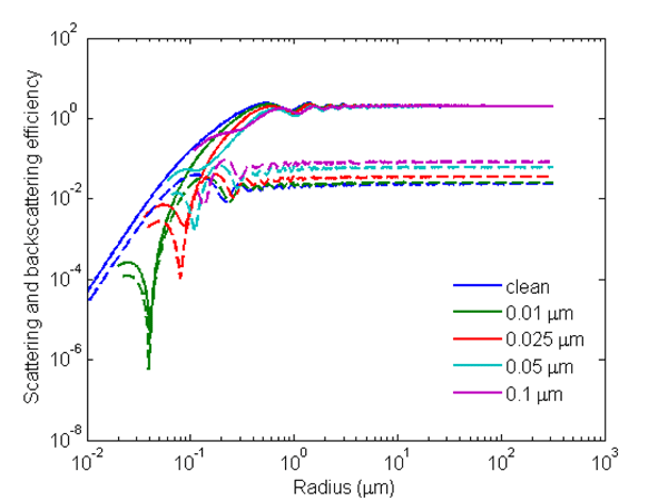
The coating of organic film on the surface of bubbles significantly affect the backscattering with little effect on the total scattering (Zhang et al. (1998)). The scattering by bubbles coated with organic film does not change very much from those by clean bubbles of sizes , but the backscattering increases with the thickness of the film, up to a factor of 4, as seen in Fig. 3. For bubbles of smaller sizes (), the coating seems to reduce both scattering and backscattering efficiency as compared to clean bubbles. There is few data on the absorption properties of films coated onto the bubble surface. The calculations assuming an imaginary part of the refractive index of values 0.001 to 0.006 showed that only when the bubble sizes reach approximately , and with extremely high absorption coefficient (imaginary index = 0.006), does absorption significantly reduce the scattering and backscattering from the case with no absorption. It is safe to say that the normally absorbing organic films exert a small influence on the scattering and backscattering of bubbles (Zhang et al. (1998)).
The bulk optical properties of bubble populations can be easily estimated once the size distribution of bubbles is known:
| (1) |
where
| (2) |
| (3) |
, and are, respectively, the mean optical efficiency factors, the mean geometric cross-sectional areas, the size distribution of the bubble population; and or , denoting total scattering or total backscattering coefficient.
Many studies attempting to characterize the size spectra of bubble populations under various stages after wave breaking have been conducted and their results are summarized in Fig. 4a. Immediately after wave breaking, the newly created bubbles are typically of sizes 0.1 - 10 mm (Deane (1997)); Haines and Johnson (1995); Phelps et al. (1997); Zhang et al. (2002)). Once bubble creation processes cease, the newly formed bubble plume evolves under the influence of turbulent diffusion, advection, buoyant degassing and dissolution, leaving behind a diffuse cloud of microbubbles (Baldy (1988); Baldy and Bourguel (1985); Breitz and Medwin (1989); Cartmill and Su (1993); Johnson and Cooke (1979); Kolovayev (1976); Leeuw and Cohen (1995); Phelps and Leighton (1998); Su and Cartmill (1994); Su et al. (1988); Terrill et al. (2001); Vagle and Farmer (1992); Vagle and Farmer (1998); Walsh and Mulhearn (1987)). Copious amounts of bubbles have also been observed in quiescent seas (Fig. 4b), sometimes with a concentration even higher than that in rough water (Huffman and Zveare (1974); Ling and Pao (1988); Medwin (1977); O’Hern et al. (1988); Shen et al. (1986)).
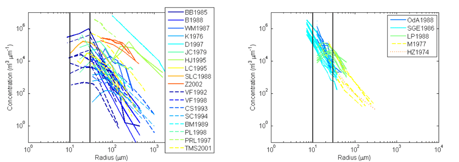
Various bubble-sensing techniques have been developed and the technology can be categorized into two groups, optics and acoustics. Optics-based methods, (solid lines in Fig. 4), include photography (Deane (1997); Johnson and Cooke (1979); Kolovayev (1976); Leeuw and Cohen (1995); Walsh and Mulhearn (1987)), light scattering and reflection (Baldy (1988); Baldy and Bourguel (1985); Ling and Pao (1988); Su et al. (1988)), and holography (O’Hern et al. (1988)). Bubbles pulsate under sound pressure and the intrinsic frequency is inversely proportional to the sizes. Bubbles of sizes that are in resonant with the acoustical frequency can significantly alter the sound propagation speed and exert an attenuation cross-section up to 100 times than those non-resonant bubbles or solid particles. The acoustics-based methods (dashed lines in Fig. 4)) include resonator (Cartmill and Su (1993); Medwin (1970); Su and Cartmill (1994); Terrill and Melville (2000); Vagle and Farmer (1998)), sound speed dispersion (Huffman and Zveare (1974)), backscatter (Vagle and Farmer (1992); Vagle and Farmer (1998)), and nonlinear interaction (Phelps and Leighton (1998); Phelps et al. (1997)).
Despite various techniques being developed and used, few studies have been able to detect bubbles of sizes (the vertical lines at in Fig. 1). We believe this limit, hardly of any natural origin, is artificial and imposed by technology being used. For acoustic frequencies greater than , which resonates with bubbles of , the off-resonant contribution from larger bubbles is very large and it is difficult to separate resonant signal from off-resonant noises. On the other hand, the size limit in photography is about -.
For bubbles of sizes , the mean optical efficiency factors are almost a constant for both scattering and backscattering (Figs. 2 and 3); therefore the bulk scattering and backscattering coefficients (Eq. 1) are determined by the size distributions. Based on the bubble size spectra shown in Fig. 4a, the natural bubble populations an account for a large portion of observed backscattering (Terrill et al. (2001); Zhang et al. (1998)) or even completely dominate the scattering process in roughened seas (Stramski and Tegowski (2001)). In clear waters, the presence of bubbles change the color of the ocean towards green (Zhang et al. (1998)).
The volume scattering functions of bubble populations were measured by a prototype volume scattering meter (Lee and Lewis (2003)) in the laboratory and the results confirmed the elevated scattering at the critical angle and the enhanced backscattering by surfactant-coated bubbles relative to the clean bubbles (Fig. 5
).
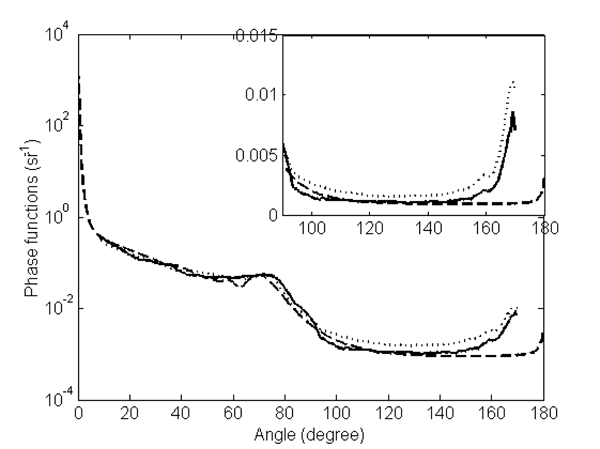
It is impossible to directly measure the volume scattering that is due to bubble populations alone in nature. However, the scattering by oceanic bubbles can be inferred from field measurement of total VSF (Zhang et al. (2002)), even though the solution might not be unique, depending directly on how well are represented of the nature of scattering by other particles and the size distribution of all particles.
Because little is known about small bubbles of sizes in nature, the optical properties of oceanic bubble populations in their entirety are still elusive. If the bubble concentration decreases at smaller sizes, then theoretical calculations and laboratory observations of the VSF for bubbles as shown in Fig. 5 are applicable to natural bubble populations; however, if the distribution is characterized by a continuous increase in the number density as size decreases (although clearly this must be bounded), then this could change the VSF in a way dependent on the size distribution of the small bubbles.
The injection of bubbles beyond the background population could significantly alter the light field both below and above the bubble layer. Being an efficient source of diffuse radiance, bubble layers contribute to a rapid transition to the diffuse asymptotic regime (Flatau et al. (1999)), and enhance and modify the spectral reflectance above the surface (Flatau et al. (2000); Piskozub et al. (2009)). Because of this, the typical ocean color algorithms for atmospheric correction (black pixel assumption) and for retrieval of the oceanic parameters (through band ratios) may no longer apply in the presence of additional bubbles (Yan et al. (2002); Zhang et al. (2004)).
 See comments posted for this page and leave your own.